Current Algebra of the HK Model

Presenter	Yuting Bai (Prof. Philip W. Phillips’s group, UIUC)
Date	August 24, 2026 · 4:30–6:00 PM
Location	Davey 339
Topic	Application of the current-algebra method to a strongly correlated problem

Current algebra asks a deceptively simple question: instead of building a many-body theory out of particles $c_{\mathbf k}, c^\dagger_{\mathbf k}$, can we build it out of the fluid variables — the densities and currents that experiments actually measure? For free fermions in one dimension the answer is the familiar $U(1)$ Kac–Moody algebra, but the standard derivation leans hard on a filled Fermi sea, a linearized dispersion and a momentum cutoff. This talk replaces that derivation with the Bjorken–Johnson–Low prescription, which extracts the equal-time commutator from the high-frequency tail of a correlation function and therefore never has to assume what the ground state looks like. Applied to the Hatsugai–Kohmoto (HK) model — an exactly solvable non-Fermi liquid that violates Luttinger’s theorem — the method shows that the natural low-energy objects are not bare currents but parton (holon/doublon) currents, that they close into an affine $\mathfrak{su}(2)$ algebra, and that a manifestly local Sugawara-type Hamiltonian built from them reproduces the HK equations of motion and two-body correlators in the infrared. The suggested moral: the notorious non-locality of the HK model may be an artifact of writing local degrees of freedom in non-local variables.

1. Two descriptions of a Fermi system

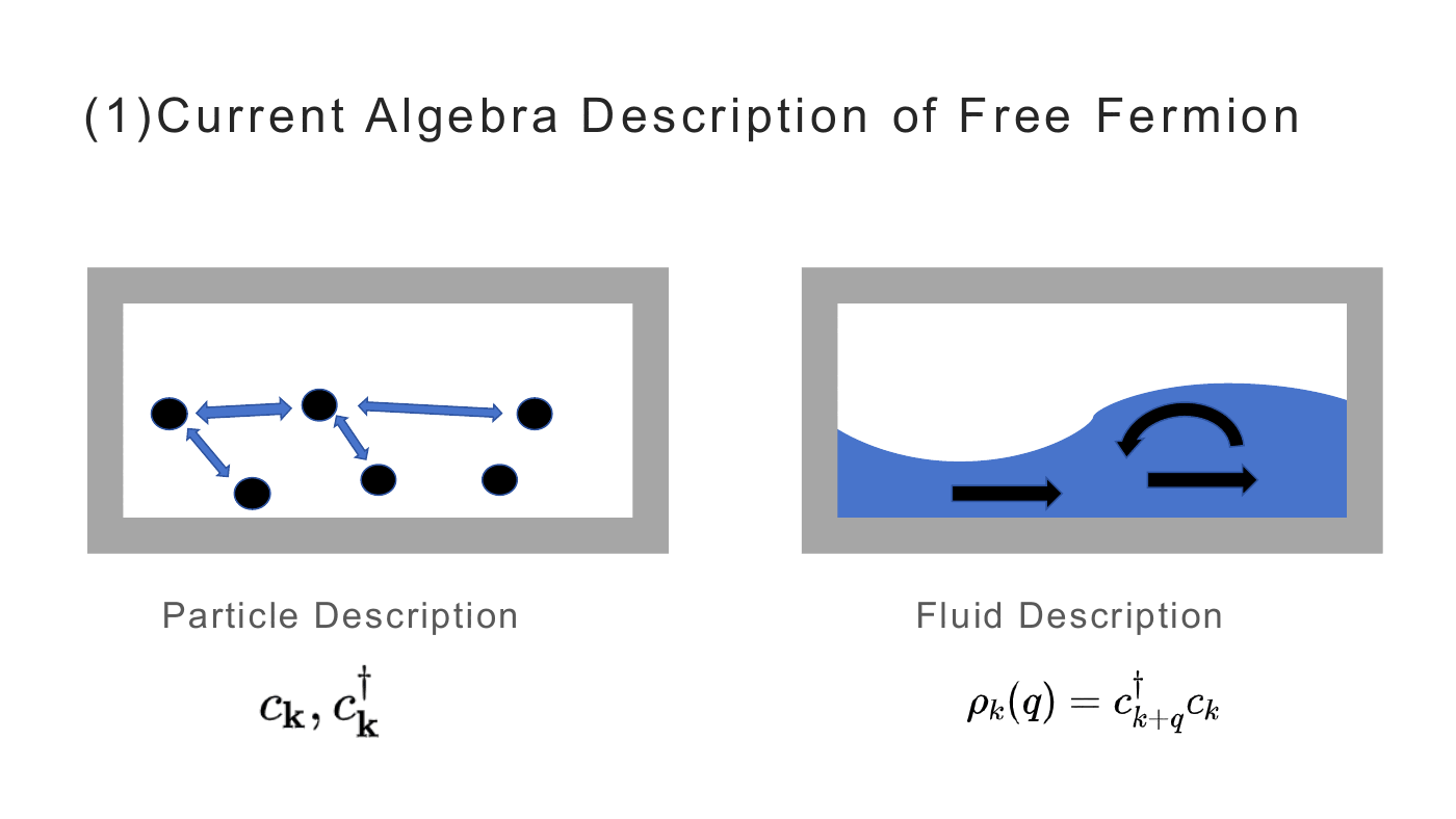
There are two inequivalent ways to name the degrees of freedom of a many-fermion system:

• Particle description — the bare operators $c_{\mathbf k},\, c^\dagger_{\mathbf k}$.

• Fluid description — the density/current bilinears

  $$ \rho_q \equiv \frac{1}{L}\int dx\, e^{iqx}\rho(x) = \sum_{\mathbf k} c^\dagger_{\mathbf k+\mathbf q} c_{\mathbf k}. $$

The fluid variables are attractive for two reasons. They are the experimentally observable objects (charge and current response), and in one dimension they close: their algebra and their equations of motion can be written without ever reintroducing $c$ and $c^\dagger$. The goal of the talk is to see how far that closure survives once interactions are switched on.

2. Current algebra of free fermions — and why the naive derivation is fragile

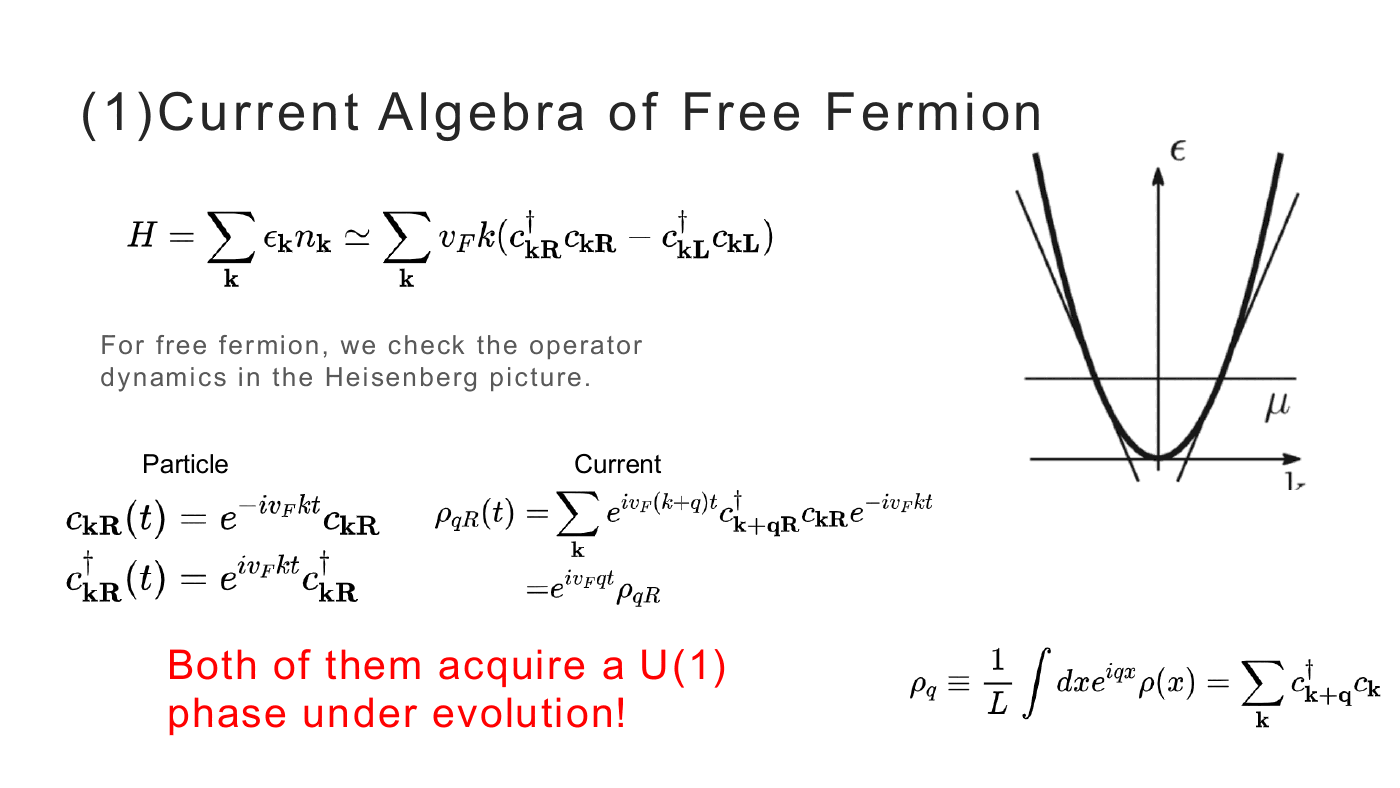
Linearize about the two Fermi points,

$$ H=\sum_{\mathbf k}\epsilon_{\mathbf k} n_{\mathbf k} \simeq \sum_{\mathbf k} v_F k\,\bigl(c^\dagger_{\mathbf k R}c_{\mathbf k R}-c^\dagger_{\mathbf k L}c_{\mathbf k L}\bigr), $$

and evolve both descriptions in the Heisenberg picture. The particle operators pick up a phase, $c_{\mathbf k R}(t)=e^{-iv_Fkt}c_{\mathbf k R}$, and so does the current,

$$ \rho_{qR}(t)=\sum_{\mathbf k}e^{iv_F(k+q)t}c^\dagger_{\mathbf k+\mathbf q R}c_{\mathbf k R}e^{-iv_Fkt} =e^{iv_Fqt}\rho_{qR}. $$

Both are eigenoperators of the time evolution — the current evolves into itself, acquiring only a $U(1)$ phase. This is exactly the property that makes a current-algebra description possible, and it is also its main limitation: it requires the dispersion to be linear and the problem to be effectively one-dimensional. Away from linearity (band edges, flat bands, higher dimensions) the current no longer evolves into itself.

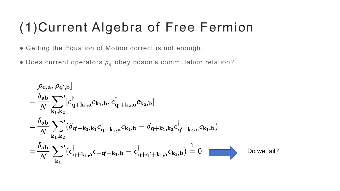
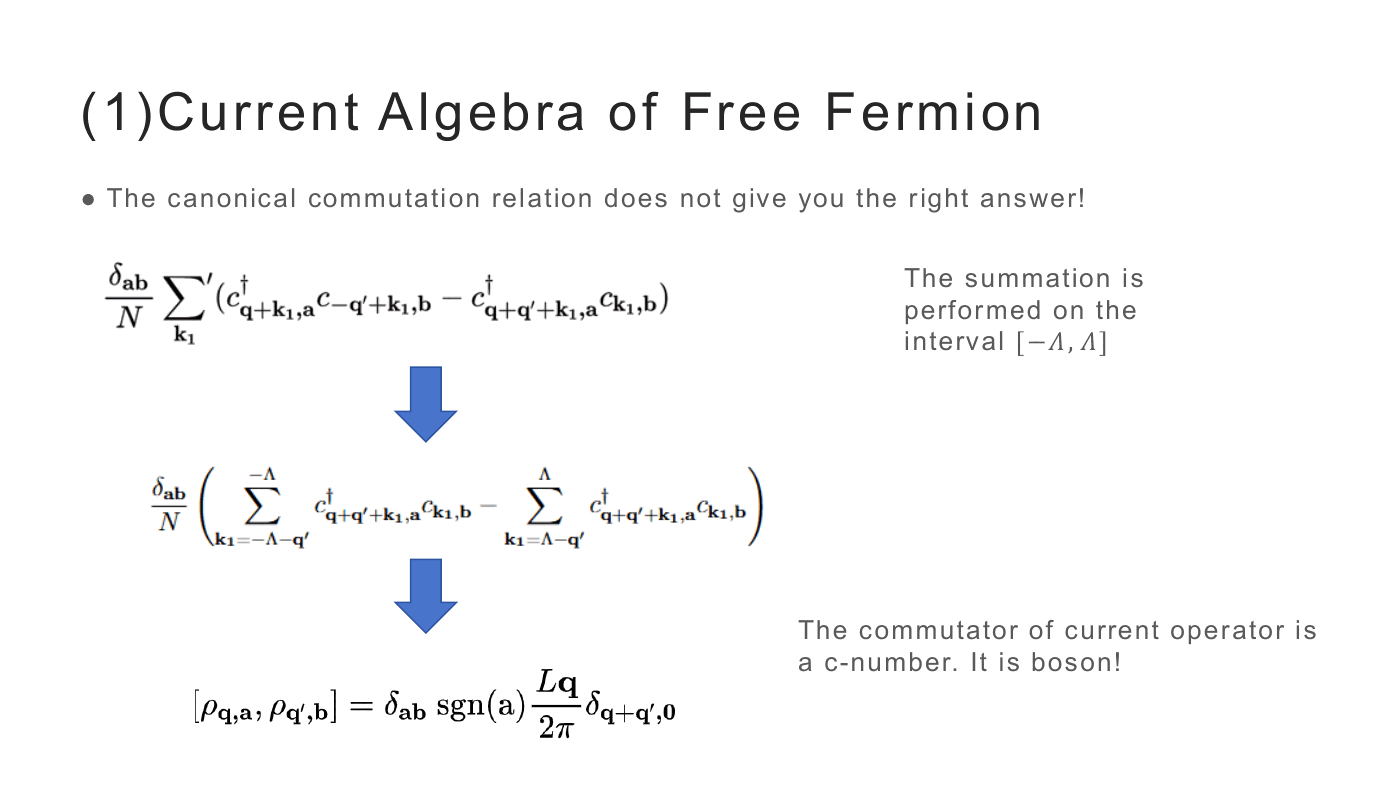
Getting the equation of motion right is not enough, though — one still has to ask whether the $\rho_q$ obey bosonic commutation relations. Manipulating the canonical anticommutators formally,

$$ [\rho_{\mathbf q,a},\rho_{\mathbf q',b}] =\frac{\delta_{ab}}{N}{\sum_{\mathbf k_1}}' \bigl(c^\dagger_{\mathbf q+\mathbf k_1,a}c_{-\mathbf q'+\mathbf k_1,b} -c^\dagger_{\mathbf q+\mathbf q'+\mathbf k_1,a}c_{\mathbf k_1,b}\bigr)\overset{?}{=}0 , $$

seems to give zero — the two sums cancel term by term. Do we fail? No: the cancellation is illegitimate because the sums run over a finite interval $[-\Lambda,\Lambda]$ and the two terms are shifted relative to one another. Keeping the boundary terms leaves

$$ \frac{\delta_{ab}}{N}\Biggl(\sum_{\mathbf k_1=-\Lambda-\mathbf q'}^{-\Lambda} c^\dagger_{\mathbf q+\mathbf q'+\mathbf k_1,a}c_{\mathbf k_1,b} -\sum_{\mathbf k_1=\Lambda-\mathbf q'}^{\Lambda} c^\dagger_{\mathbf q+\mathbf q'+\mathbf k_1,a}c_{\mathbf k_1,b}\Biggr) $$

which, evaluated in the filled sea, is the Schwinger term

$$ [\rho_{\mathbf q,a},\rho_{\mathbf q',b}]=\delta_{ab}\,\mathrm{sgn}(a)\,\frac{Lq}{2\pi}\,\delta_{\mathbf q+\mathbf q',0}. $$

The commutator is a $c$-number: the currents are bosons. The catch is that this anomaly was extracted from a cutoff-dependent boundary term evaluated on a free filled Fermi sea. That is not a derivation one can trust in an interacting problem.

3. The Bjorken–Johnson–Low prescription

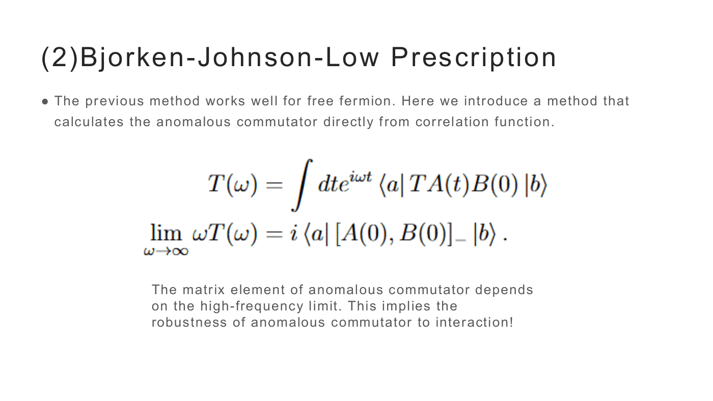
The fix is to compute the anomalous commutator directly from a correlation function. For any two operators $A$, $B$, define the time-ordered correlator

$$ T(\omega)=\int dt\, e^{i\omega t}\,\langle a|\,T A(t)B(0)\,|b\rangle , $$

then the BJL prescription reads the equal-time commutator off its high-frequency tail:

$$ \lim_{\omega\to\infty}\omega\,T(\omega)=i\,\langle a|\,[A(0),B(0)]_-\,|b\rangle . $$

Two things make this the right tool here. First, it is a statement about the UV behaviour of the correlator, so the commutator it produces is insensitive to the infrared details — the ground state need not be assumed to be a Fermi sea. Second, and for the same reason, the anomalous commutator inherits a certain robustness against interactions: whatever the interaction does to the low-energy physics, it does not change the $\omega\to\infty$ tail that fixes the algebra. (This was also the point of the closing discussion — see §10.)

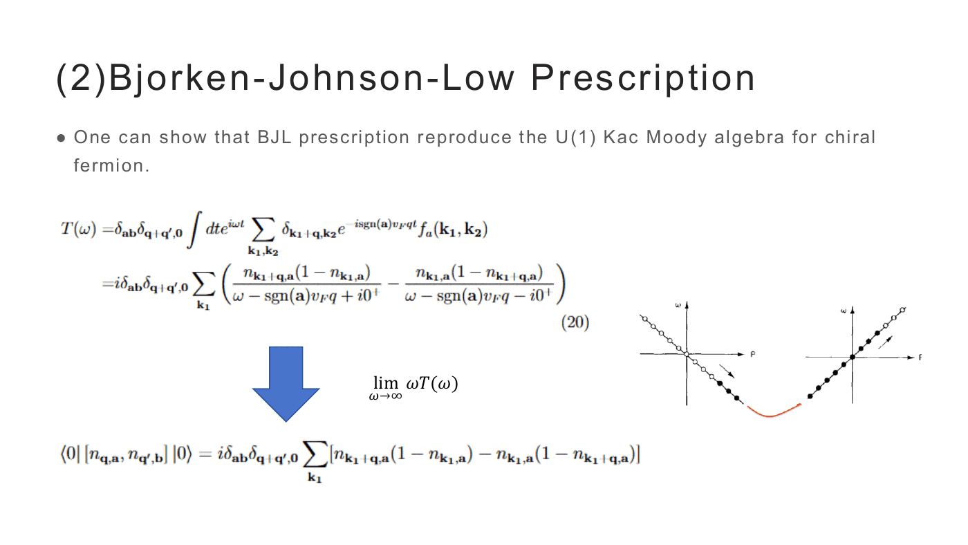
As a check, applying BJL to chiral fermions reproduces the $U(1)$ Kac–Moody algebra. Writing

$$ T(\omega)=i\delta_{ab}\delta_{\mathbf q+\mathbf q',0}\sum_{\mathbf k_1} \left(\frac{n_{\mathbf k_1+\mathbf q,a}(1-n_{\mathbf k_1,a})}{\omega-\mathrm{sgn}(a)v_Fq+i0^+} -\frac{n_{\mathbf k_1,a}(1-n_{\mathbf k_1+\mathbf q,a})}{\omega-\mathrm{sgn}(a)v_Fq-i0^+}\right) $$

and taking $\lim_{\omega\to\infty}\omega T(\omega)$ gives

$$ \langle 0|\,[n_{\mathbf q,a},n_{\mathbf q',b}]\,|0\rangle =i\delta_{ab}\delta_{\mathbf q+\mathbf q',0}\sum_{\mathbf k_1} \bigl[n_{\mathbf k_1+\mathbf q,a}(1-n_{\mathbf k_1,a})-n_{\mathbf k_1,a}(1-n_{\mathbf k_1+\mathbf q,a})\bigr], $$

i.e. the same Schwinger term, now obtained without any cutoff bookkeeping.

4. Could interaction change the current algebra?

If Luttinger’s theorem holds, the low-energy dynamics of a Fermi surface is that of an incompressible droplet — the coadjoint-orbit / nonlinear-bosonization picture of Delacrétaz, Du, Mehta and Son. In that case the current algebra is essentially fixed by geometry and one should not expect interactions to modify it. The natural place to look for a violation is therefore a system in which Luttinger’s theorem itself fails.

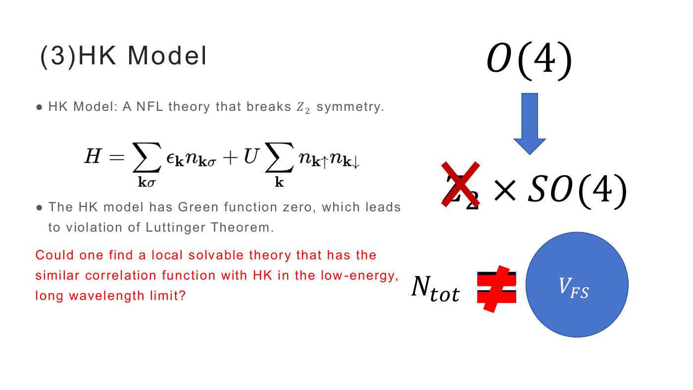
A complementary way to say the same thing: a Fermi liquid enjoys an $O(4)$ symmetry, whose discrete part is a $\mathbb{Z}_2$. A generic interaction $\sum_{k\sigma,q\sigma'} f^{\sigma\sigma'}_{k,q} n_{k\sigma}n_{q\sigma'}$ breaks that $\mathbb{Z}_2$ — yet the Fermi liquid is stable against it. Are there stable fixed points that break the $\mathbb{Z}_2$? The HK model is the simplest place to find out.

5. The HK model

$$ H=\sum_{\mathbf k\sigma}\epsilon_{\mathbf k}n_{\mathbf k\sigma}+U\sum_{\mathbf k}n_{\mathbf k\uparrow}n_{\mathbf k\downarrow}. $$

The Hatsugai–Kohmoto interaction is diagonal in momentum, which makes the model exactly solvable in any dimension while remaining a genuine non-Fermi liquid: its Green function has zeros, the Luttinger count fails ($N_{\rm tot}\neq V_{\rm FS}$), and the $O(4)\simeq\mathbb{Z}_2\times SO(4)$ of the Fermi liquid loses its discrete factor, leaving $SO(4)$ — precisely the $\mathbb{Z}_2$-breaking fixed point we were looking for.

The organizing question of the talk:

Can one find a local, solvable theory with the same correlation functions as HK in the low-energy, long-wavelength limit?

6. Parton currents: holons and doublons

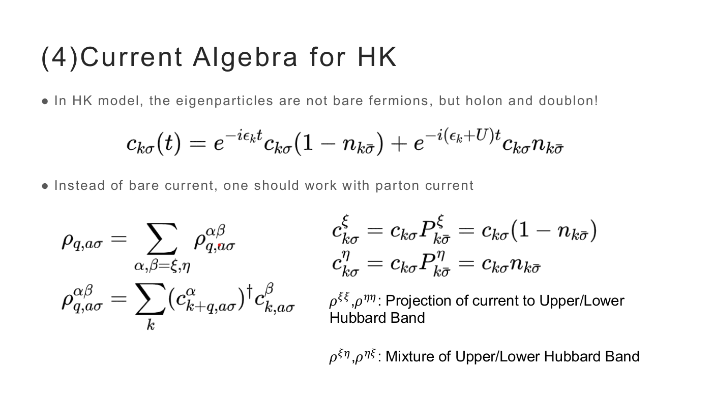
In the HK model the eigen-operators of the time evolution are not the bare fermions:

$$ c_{k\sigma}(t)=e^{-i\epsilon_k t}c_{k\sigma}(1-n_{k\bar\sigma})+e^{-i(\epsilon_k+U)t}c_{k\sigma}n_{k\bar\sigma}. $$

The bare $c$ splits into a holon and a doublon, evolving with $\epsilon_k$ and $\epsilon_k+U$ respectively. So one should work not with the bare current but with the parton current. Define the projected operators

$$ c^{\xi}_{k\sigma}=c_{k\sigma}P^{\xi}_{k\bar\sigma}=c_{k\sigma}(1-n_{k\bar\sigma}),\qquad c^{\eta}_{k\sigma}=c_{k\sigma}P^{\eta}_{k\bar\sigma}=c_{k\sigma}n_{k\bar\sigma}, $$

and the associated currents

$$ \rho_{q,a\sigma}=\sum_{\alpha,\beta=\xi,\eta}\rho^{\alpha\beta}_{q,a\sigma}, \qquad \rho^{\alpha\beta}_{q,a\sigma}=\sum_k \bigl(c^{\alpha}_{k+q,a\sigma}\bigr)^\dagger c^{\beta}_{k,a\sigma}. $$

Here $\rho^{\xi\xi}$ and $\rho^{\eta\eta}$ are the currents projected onto the lower and upper Hubbard band, while $\rho^{\xi\eta}$ and $\rho^{\eta\xi}$ mix the two bands.

7. The algebra, from BJL

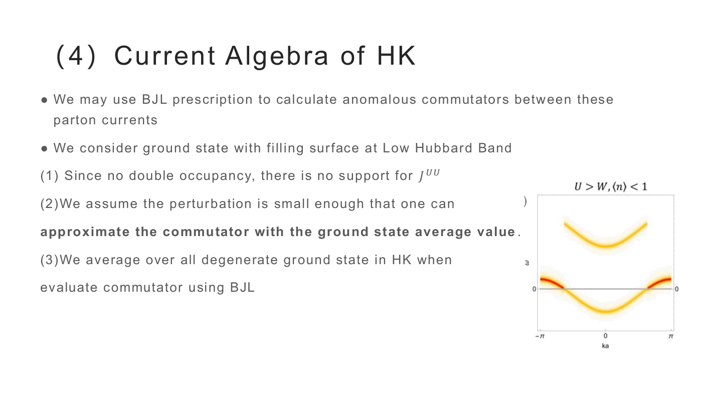
Take the ground state with the filling surface in the lower Hubbard band, and note three working assumptions:

1. With no double occupancy there is no support for $J^{UU}$.
2. The perturbation is weak enough that the commutator may be approximated by its ground-state expectation value.
3. One averages over the (massively degenerate) HK ground-state manifold when evaluating the BJL limit.

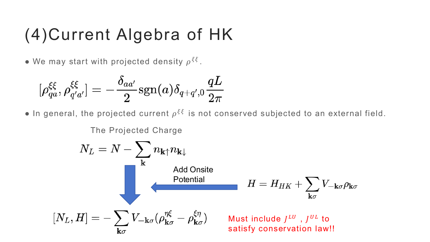
The projected density then obeys a halved Schwinger term,

$$ \bigl[\rho^{\xi\xi}_{qa},\rho^{\xi\xi}_{q'a'}\bigr] =-\frac{\delta_{aa'}}{2}\,\mathrm{sgn}(a)\,\delta_{q+q',0}\,\frac{qL}{2\pi}. $$

But the projected current is not conserved in the presence of an external field. With the projected charge $N_L=N-\sum_{\mathbf k}n_{\mathbf k\uparrow}n_{\mathbf k\downarrow}$ and an added onsite potential $H=H_{HK}+\sum_{\mathbf k\sigma}V_{-\mathbf k\sigma}\rho_{\mathbf k\sigma}$,

$$ [N_L,H]=-\sum_{\mathbf k\sigma}V_{-\mathbf k\sigma}\bigl(\rho^{\eta\xi}_{\mathbf k\sigma}-\rho^{\xi\eta}_{\mathbf k\sigma}\bigr)\neq 0 , $$

so the interband currents $J^{LU}$, $J^{UL}$ must be included for the conservation law to hold. The full algebra is

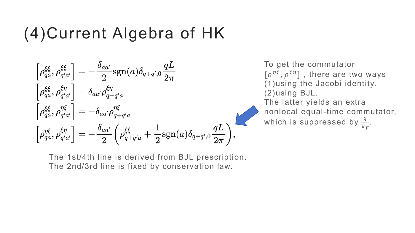
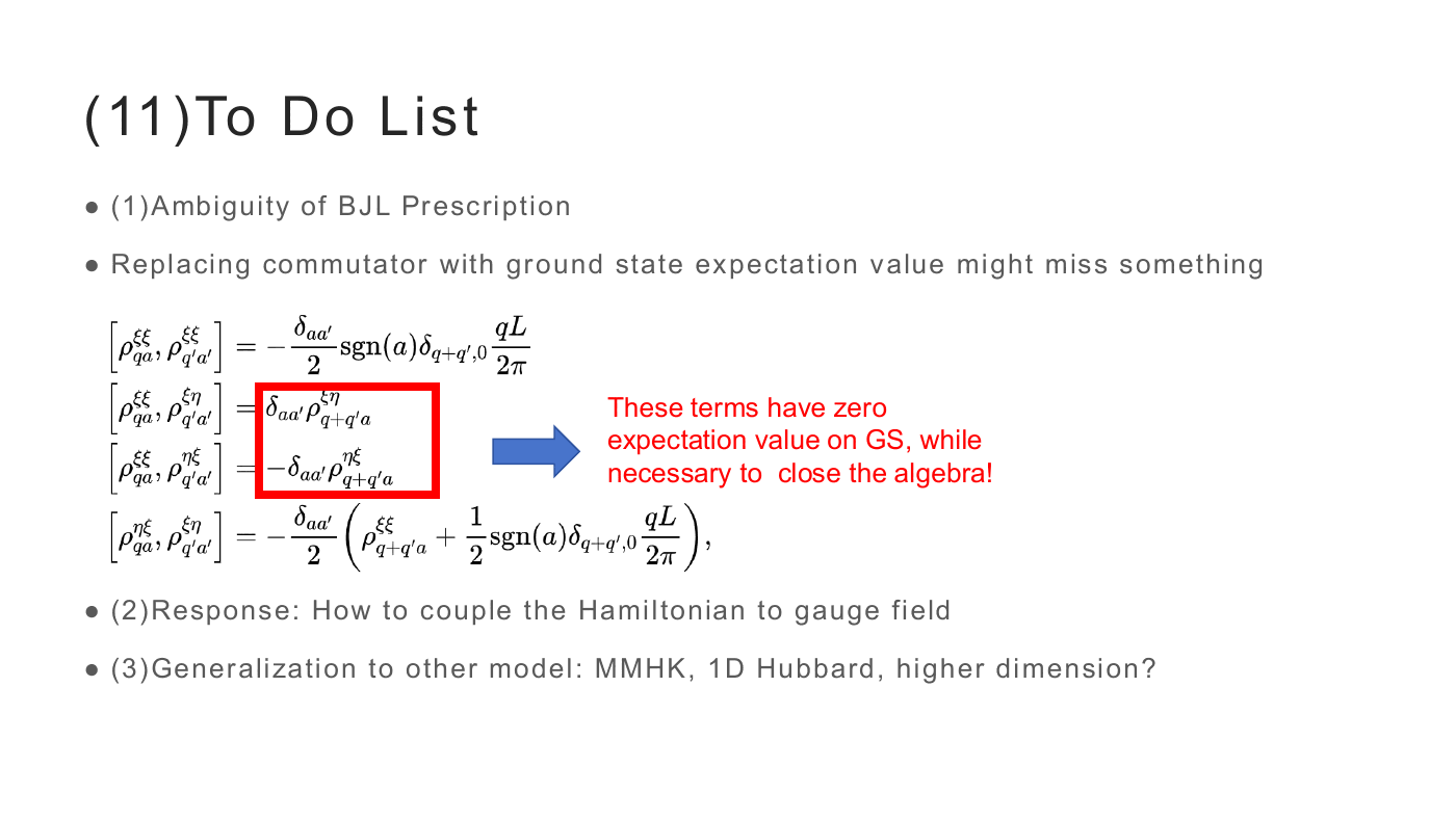
$$ \bigl[\rho^{\xi\xi}_{qa},\rho^{\xi\xi}_{q'a'}\bigr]=-\frac{\delta_{aa'}}{2}\mathrm{sgn}(a)\delta_{q+q',0}\frac{qL}{2\pi}, \qquad \bigl[\rho^{\xi\xi}_{qa},\rho^{\xi\eta}_{q'a'}\bigr]=\delta_{aa'}\rho^{\xi\eta}_{q+q'a}, $$$$ \bigl[\rho^{\xi\xi}_{qa},\rho^{\eta\xi}_{q'a'}\bigr]=-\delta_{aa'}\rho^{\eta\xi}_{q+q'a}, \qquad \bigl[\rho^{\eta\xi}_{qa},\rho^{\xi\eta}_{q'a'}\bigr] =-\frac{\delta_{aa'}}{2}\Bigl(\rho^{\xi\xi}_{q+q'a}+\frac{1}{2}\mathrm{sgn}(a)\delta_{q+q',0}\frac{qL}{2\pi}\Bigr), $$

where the first and fourth lines come from BJL and the second and third are fixed by the conservation law. (The last commutator can also be obtained from the Jacobi identity; BJL instead yields an extra non-local equal-time piece, suppressed by $q/k_F$.)

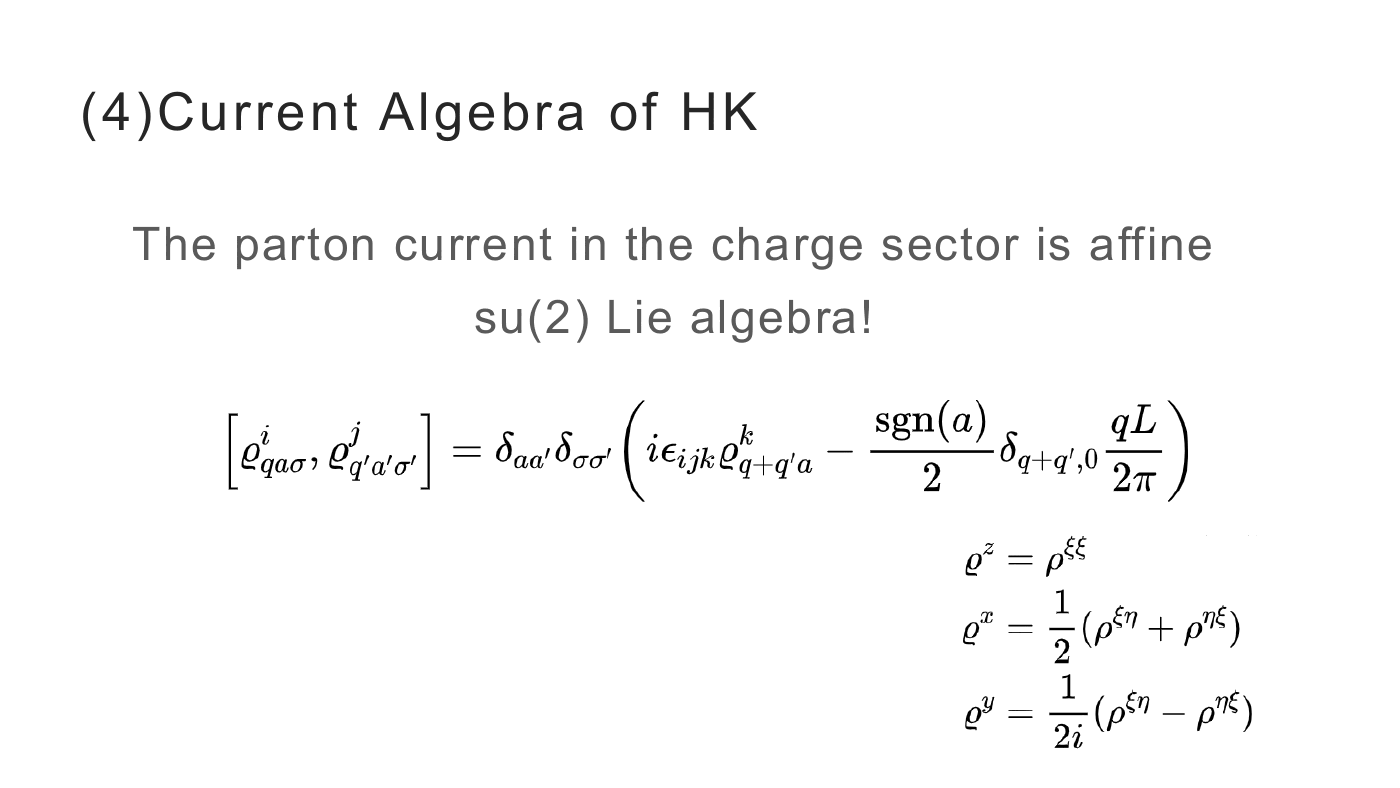
8. Affine su(2)

Assembling the currents into a triplet,

$$ \varrho^{z}=\rho^{\xi\xi},\qquad \varrho^{x}=\tfrac{1}{2}\bigl(\rho^{\xi\eta}+\rho^{\eta\xi}\bigr),\qquad \varrho^{y}=\tfrac{1}{2i}\bigl(\rho^{\xi\eta}-\rho^{\eta\xi}\bigr), $$

the whole algebra collapses into a single line:

$$ \bigl[\varrho^{i}_{qa\sigma},\varrho^{j}_{q'a'\sigma'}\bigr] =\delta_{aa'}\delta_{\sigma\sigma'}\Bigl(i\epsilon_{ijk}\varrho^{k}_{q+q'a} -\frac{\mathrm{sgn}(a)}{2}\delta_{q+q',0}\frac{qL}{2\pi}\Bigr). $$

The parton current in the charge sector realizes an affine $\mathfrak{su}(2)$ Lie algebra — an $SU(2)$ structure with a central (Schwinger) extension. This is the central result of the talk: interaction has not destroyed the current algebra, it has enlarged it, from $U(1)$ Kac–Moody to affine $\mathfrak{su}(2)$.

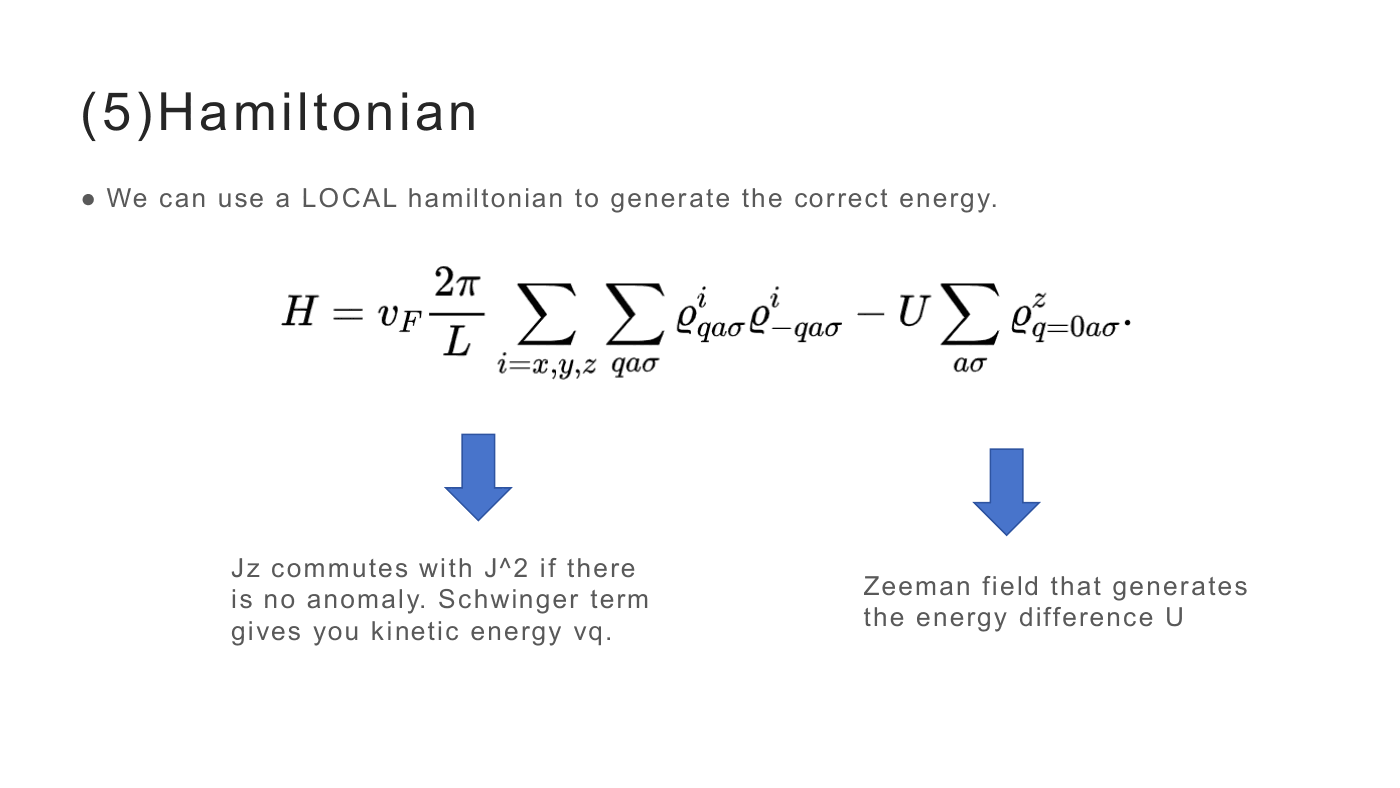
9. A local Hamiltonian from the algebra

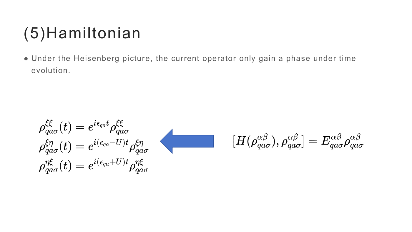
Under Heisenberg evolution each parton current is again an eigenoperator,

$$ \rho^{\xi\xi}_{qa\sigma}(t)=e^{i\epsilon_{qa}t}\rho^{\xi\xi}_{qa\sigma},\quad \rho^{\xi\eta}_{qa\sigma}(t)=e^{i(\epsilon_{qa}-U)t}\rho^{\xi\eta}_{qa\sigma},\quad \rho^{\eta\xi}_{qa\sigma}(t)=e^{i(\epsilon_{qa}+U)t}\rho^{\eta\xi}_{qa\sigma}, $$

i.e. $[H(\rho^{\alpha\beta}_{qa\sigma}),\rho^{\alpha\beta}_{qa\sigma}]=E^{\alpha\beta}_{qa\sigma}\rho^{\alpha\beta}_{qa\sigma}$. Any Hamiltonian reproducing these three eigenvalues reproduces the HK equations of motion — and one can be built entirely out of the currents, Sugawara-style:

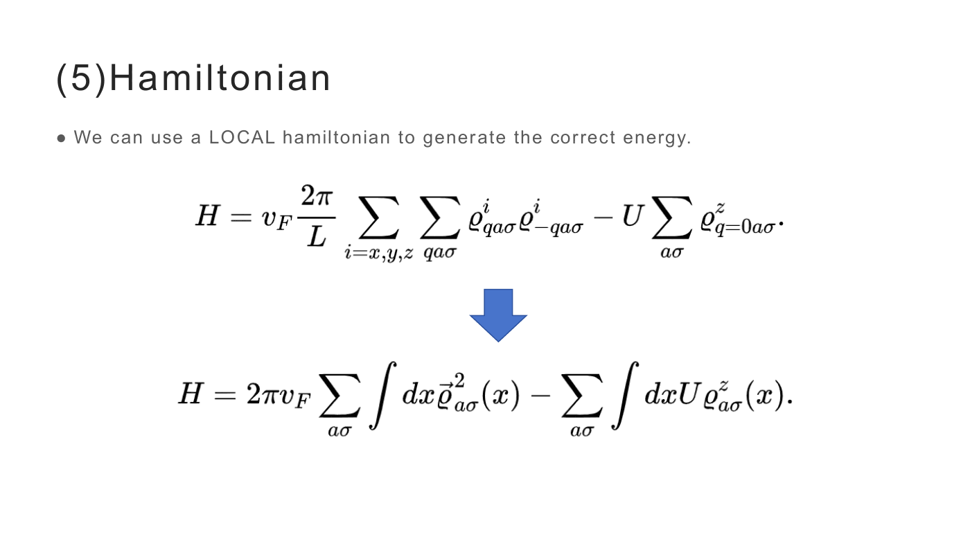
$$ H=v_F\frac{2\pi}{L}\sum_{i=x,y,z}\sum_{qa\sigma}\varrho^{i}_{qa\sigma}\varrho^{i}_{-qa\sigma} -U\sum_{a\sigma}\varrho^{z}_{q=0,a\sigma}. $$

The first term is the Casimir $\vec{\varrho}^{\,2}$: $\varrho^z$ commutes with it in the absence of the anomaly, and it is precisely the Schwinger term that converts the Casimir into the kinetic energy $v_Fq$. The second term acts as a Zeeman field that generates the holon–doublon splitting $U$. In real space,

$$ H=2\pi v_F\sum_{a\sigma}\int dx\,\vec{\varrho}^{\,2}_{a\sigma}(x)-\sum_{a\sigma}\int dx\, U\varrho^{z}_{a\sigma}(x), $$

which is manifestly local — a local Hamiltonian reproducing the dynamics of a model usually described as non-local.

10. Geometry and topology

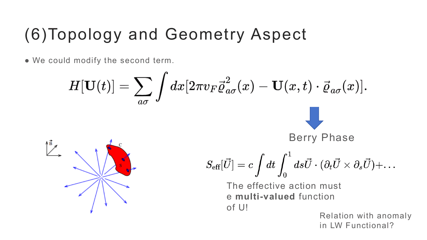
Promoting the “Zeeman field” to a spacetime-dependent vector,

$$ H[\mathbf U(t)]=\sum_{a\sigma}\int dx\,\bigl[2\pi v_F\vec{\varrho}^{\,2}_{a\sigma}(x)-\mathbf U(x,t)\cdot\vec{\varrho}_{a\sigma}(x)\bigr], $$

the resulting effective action carries a Berry-phase (Wess–Zumino-like) term

$$ S_{\rm eff}[\vec U]=c\int dt\int_0^1 ds\,\vec U\cdot\bigl(\partial_t\vec U\times\partial_s\vec U\bigr)+\dots $$

which forces $S_{\rm eff}$ to be a multi-valued functional of $\vec U$ — the familiar spin-coherent-state structure, with the extra parameter $s$ interpolating to a reference configuration. An open question raised here: is this the same anomaly that shows up in the Luttinger–Ward functional?

11. Does it actually reproduce HK?

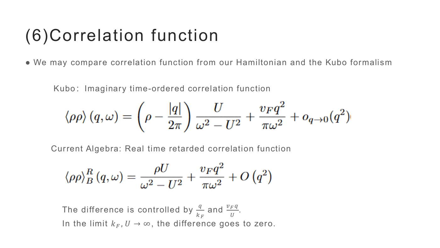
Compare the density–density correlator computed two ways. From Kubo (imaginary-time-ordered) on the HK model,

$$ \langle\rho\rho\rangle(q,\omega)=\Bigl(\rho-\frac{|q|}{2\pi}\Bigr)\frac{U}{\omega^2-U^2} +\frac{v_Fq^2}{\pi\omega^2}+o_{q\to0}(q^2), $$

and from the current-algebra Hamiltonian (real-time retarded),

$$ \langle\rho\rho\rangle^{R}_{B}(q,\omega)=\frac{\rho U}{\omega^2-U^2}+\frac{v_Fq^2}{\pi\omega^2}+O(q^2). $$

The two agree up to terms controlled by $q/k_F$ and $v_Fq/U$; in the limit $k_F,\,U\to\infty$ the difference vanishes. The local theory is therefore an honest IR-equivalent description, not an exact rewriting.

12. A new reading of the HK model

Three claims close the talk:

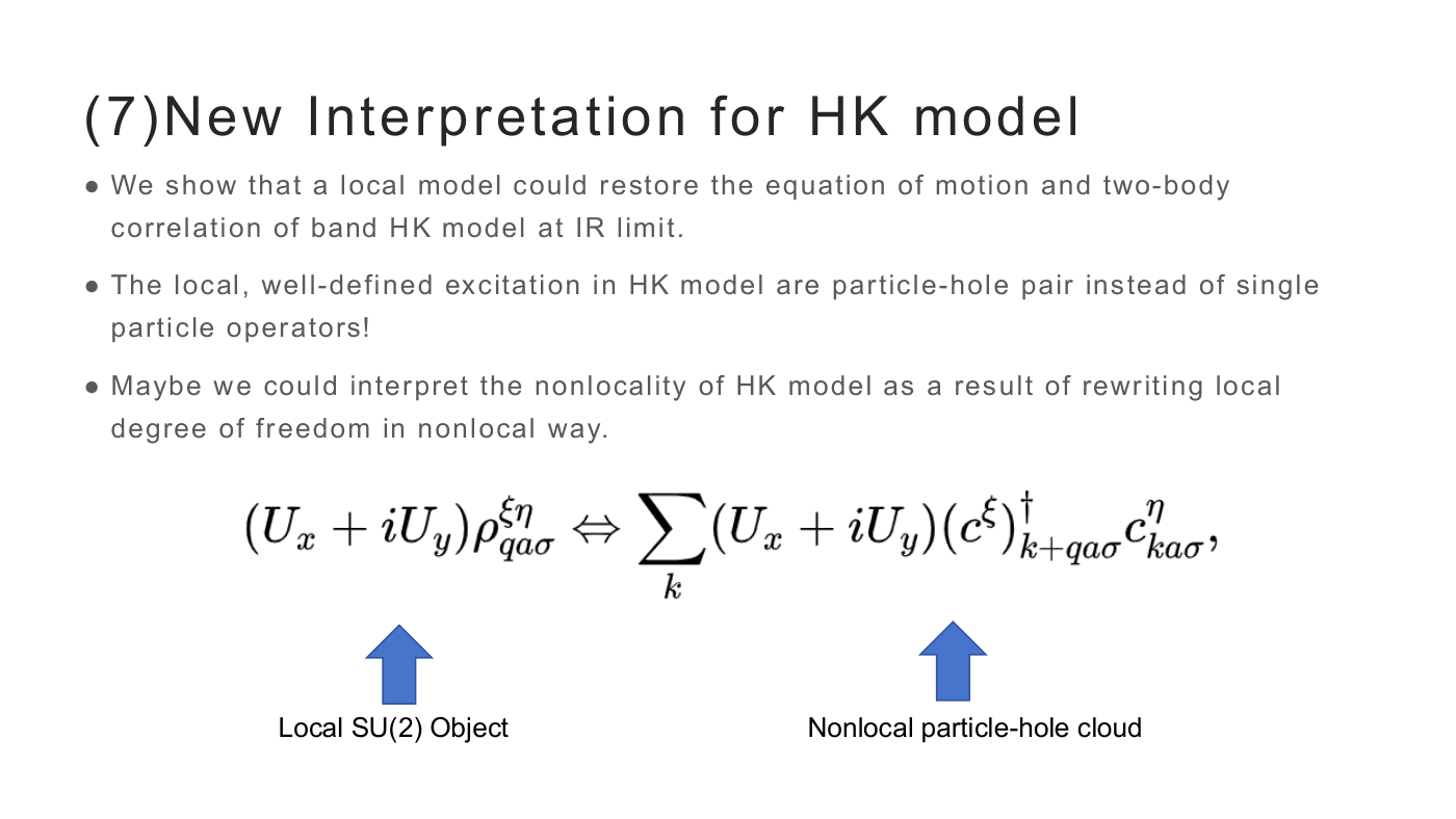
• A local model restores the equations of motion and the two-body correlators of the band HK model in the IR limit.

• The well-defined local excitations of the HK model are particle–hole pairs, not single-particle operators.

• The notorious non-locality of HK may be an artifact of variables — a local degree of freedom rewritten in a non-local way:

  $$ (U_x+iU_y)\rho^{\xi\eta}_{qa\sigma}\;\Longleftrightarrow\; \sum_k (U_x+iU_y)\bigl(c^{\xi}\bigr)^\dagger_{k+qa\sigma}c^{\eta}_{ka\sigma}, $$

  where the left-hand side is a local $SU(2)$ object and the right-hand side is a non-local particle–hole cloud. Same physics, different bookkeeping.

13. To-do list

1. Ambiguity of the BJL prescription. Replacing the commutator by its ground-state expectation value may miss operators that have zero expectation value in the ground state but are nevertheless necessary to close the algebra — exactly the interband terms $[\rho^{\xi\xi},\rho^{\xi\eta}]$ and $[\rho^{\xi\xi},\rho^{\eta\xi}]$ above.
2. Response. How should the current-algebra Hamiltonian be coupled to a gauge field?
3. Generalization. MMHK, the 1D Hubbard model, higher dimensions.
4. Quantify the residual gap between the low-energy effective theory and HK, and pin down the geometric-phase structure of §10.

Discussion points

• Why does a high-frequency limit control the low-energy algebra? The equal-time commutator is a UV-determined object, which is what makes BJL usable without assuming the ground state; the algebra it fixes then constrains the IR theory rather than being derived from it.
• What does an external magnetic field do to the current algebra? — raised in the discussion; it bears directly on to-do item 2 (coupling to a gauge field).
• What does the current operator give when acting on an occupied state? The parton projections make this question sharper than in the free case, and the answer is tied to the Casimir structure of the Sugawara Hamiltonian.
• Relation to older bosonization schemes. Formally the construction resembles the Tomonaga-style linearization-plus-boson-approximation, but the motivation is different: here the algebra is extracted from correlation functions rather than assumed, and the spectrum follows from the Casimir rather than from a postulated bosonic Hamiltonian.
• Where the description must break. The current evolves into itself only for a linear dispersion in one dimension; flat bands, band edges/tops, and higher dimensions are all open, and the momentum sums are meaningful only inside the linearization window $|k|<\Lambda$.

References

1. Y. Hatsugai and M. Kohmoto, “Exactly solvable model of correlated lattice electrons in any dimensions,” J. Phys. Soc. Jpn. 61, 2056 (1992).
2. P. W. Phillips, L. Yeo and E. W. Huang, “Exact theory for superconductivity in a doped Mott insulator,” Nat. Phys. 16, 1175 (2020).
3. L. V. Delacrétaz, Y.-H. Du, U. Mehta and D. T. Son, “Nonlinear bosonization of Fermi surfaces: The method of coadjoint orbits,” Phys. Rev. Research 4, 033131 (2022).
4. J. D. Bjorken, “Applications of the chiral $U(6)\otimes U(6)$ algebra of current densities,” Phys. Rev. 148, 1467 (1966).
5. K. Johnson and F. E. Low, “Current algebras in a simple model,” Prog. Theor. Phys. Suppl. 37–38, 74 (1966).
6. J. Schwinger, “Field theory commutators,” Phys. Rev. Lett. 3, 296 (1959).
7. D. C. Mattis and E. H. Lieb, “Exact solution of a many-fermion system and its associated boson field,” J. Math. Phys. 6, 304 (1965).