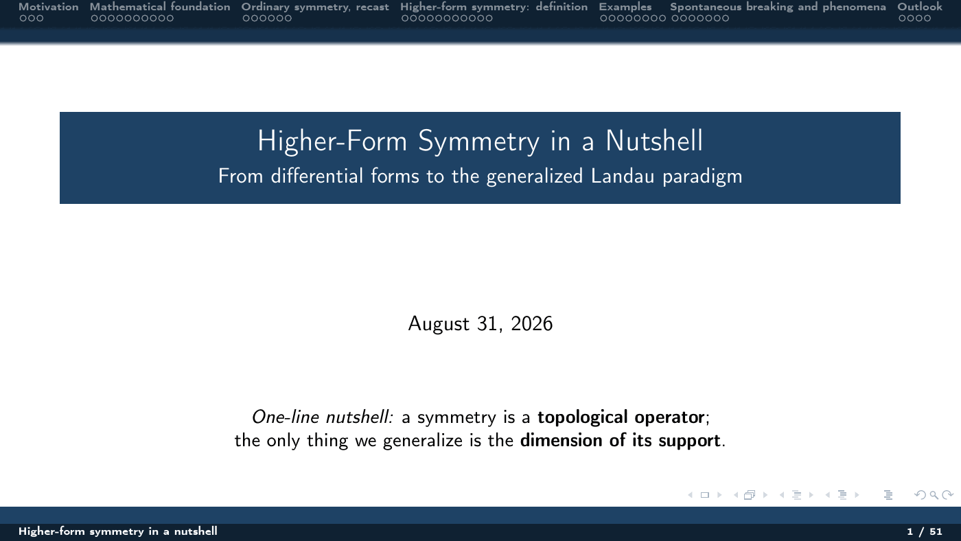
Higher-Form Symmetry in a Nutshell

Presenter	Jinfei Zhou (Prof. Zhen Bi’s group, Penn State)
Date	August 31, 2026 · 5:00–6:00 PM — continued September 7, 2026 · 4:30–6:00 PM
Location	Davey 339
Topic	Higher-form symmetry — from differential forms to the generalized Landau paradigm

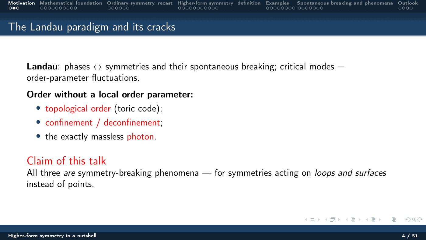
Landau’s paradigm says a phase is labelled by a symmetry and how it breaks, and that the critical modes are order-parameter fluctuations. Three familiar things appear to escape it: topological order, confinement/deconfinement, and the exact masslessness of the photon — none of them has a local order parameter. The claim of this talk is that all three are symmetry-breaking phenomena, once you allow the symmetry to act on loops and surfaces rather than on points. The route there is a single conceptual pivot: a symmetry is not a transformation of the fields but a topological operator supported on a submanifold, and the only thing being generalized is the dimension of that support. Two sessions took the argument from differential forms and linking numbers, through the recasting of ordinary Noether symmetry as a codimension-1 defect, to the definition of $p$-form symmetry and its realizations in Maxwell theory, the toric code, $\mathbb{Z}_N$ gauge theory, Chern–Simons theory and the $\mathbb{Z}_N$ center of Yang–Mills — ending with generalized order parameters, the photon as a Goldstone boson, a higher-form Mermin–Wagner theorem, and ’t Hooft anomalies.

Part 1 — Motivation: where Landau cracks

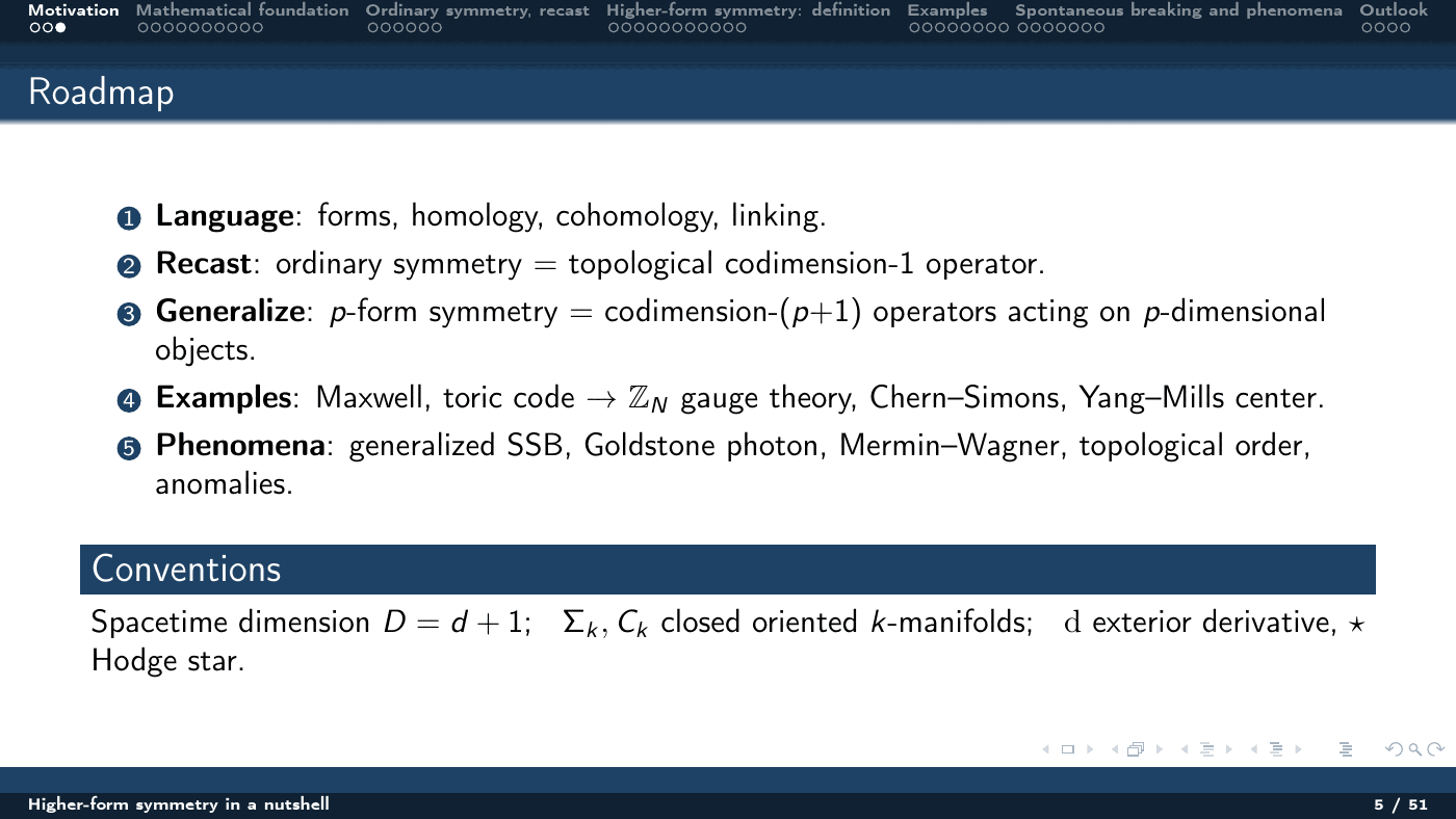
Landau’s programme is a dictionary: phases $\leftrightarrow$ symmetries and their spontaneous breaking, with the critical modes identified as fluctuations of the order parameter. The well-known failures are all cases of order without a local order parameter:

• topological order (the toric code and its ground-state degeneracy),
• confinement versus deconfinement in gauge theory,
• the exactly massless photon.

The talk’s thesis is that these are not “beyond Landau” at all — they are Landau’s story told for symmetries whose charged objects are extended.

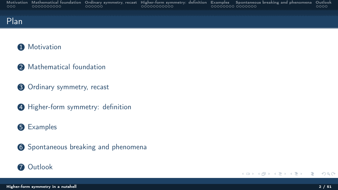
The roadmap is four steps, and it is worth keeping in view because every later slide is one of them:

1. Language — forms, homology, cohomology, linking.
2. Recast — ordinary symmetry $=$ topological codimension-1 operator.
3. Generalize — a $p$-form symmetry has codimension-$(p+1)$ operators acting on $p$-dimensional objects.
4. Examples and phenomena — Maxwell, toric code, $\mathbb{Z}_N$ gauge theory, Chern–Simons, Yang–Mills center; then generalized SSB, the Goldstone photon, Mermin–Wagner, topological order, anomalies.

Conventions throughout: spacetime dimension $D = d+1$; $\Sigma_k, C_k$ are closed oriented $k$-manifolds; $\mathrm{d}$ is the exterior derivative and $\star$ the Hodge star.

Part 2 — The mathematics, kept to a minimum

Forms, wedge, exterior derivative

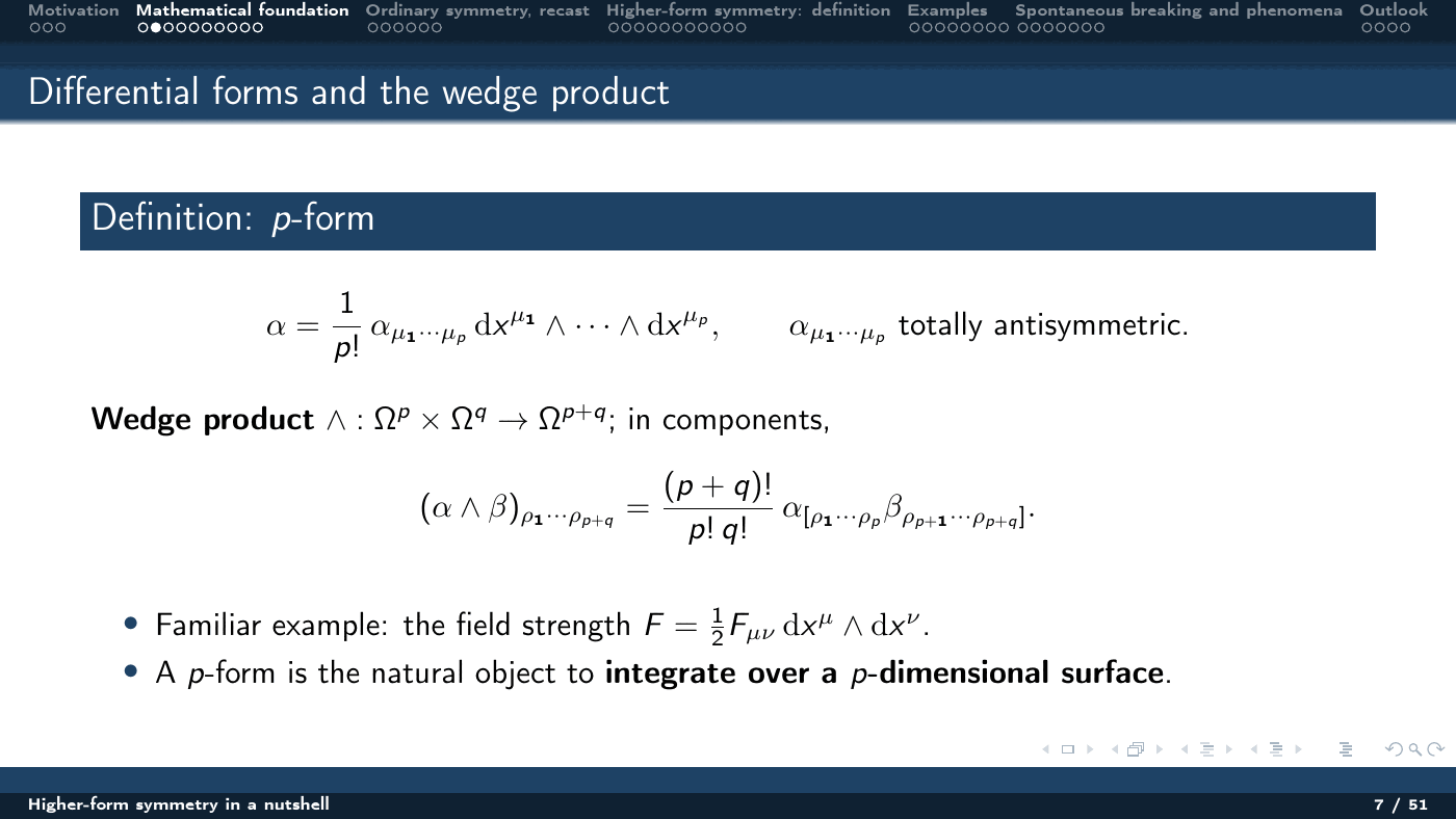
A $p$-form is

$$ \alpha = \frac{1}{p!}\,\alpha_{\mu_1\cdots\mu_p}\, \mathrm{d}x^{\mu_1}\wedge\cdots\wedge\mathrm{d}x^{\mu_p}, $$

with $\alpha_{\mu_1\cdots\mu_p}$ totally antisymmetric, and the wedge product $\wedge:\Omega^p\times\Omega^q\to\Omega^{p+q}$ acts in components as

$$ (\alpha\wedge\beta)_{\rho_1\cdots\rho_{p+q}} = \frac{(p+q)!}{p!\,q!}\,\alpha_{[\rho_1\cdots\rho_p}\beta_{\rho_{p+1}\cdots\rho_{p+q}]}. $$

The familiar example is the field strength $F = \tfrac12 F_{\mu\nu}\mathrm{d}x^\mu\wedge \mathrm{d}x^\nu$. The point to hold on to: a $p$-form is the natural object to integrate over a $p$-dimensional surface.

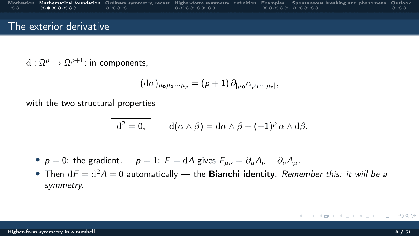
The exterior derivative $\mathrm{d}:\Omega^p\to\Omega^{p+1}$, $(\mathrm{d}\alpha)_{\mu_0\mu_1\cdots\mu_p} = (p+1)\,\partial_{[\mu_0}\alpha_{\mu_1\cdots\mu_p]}$, satisfies

$$ \mathrm{d}^2 = 0, \qquad \mathrm{d}(\alpha\wedge\beta) = \mathrm{d}\alpha\wedge\beta + (-1)^p\alpha\wedge\mathrm{d}\beta . $$

At $p=0$ this is the gradient; at $p=1$, $F = \mathrm{d}A$ reproduces $F_{\mu\nu} = \partial_\mu A_\nu - \partial_\nu A_\mu$, and then $\mathrm{d}F = \mathrm{d}^2 A = 0$ automatically — the Bianchi identity. Remember that one: it will turn out to be a symmetry.

Hodge star, and where codimension comes from

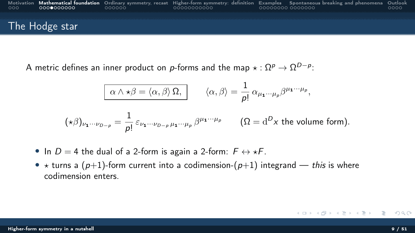
A metric gives an inner product on $p$-forms and the map $\star:\Omega^p\to\Omega^{D-p}$,

$$ \alpha\wedge\star\beta = \langle\alpha,\beta\rangle\,\Omega,\qquad \langle\alpha,\beta\rangle = \frac{1}{p!}\alpha_{\mu_1\cdots\mu_p}\beta^{\mu_1\cdots\mu_p}, $$

with $\Omega = \mathrm{d}^Dx$ the volume form. In $D=4$ the dual of a 2-form is again a 2-form, $F\leftrightarrow\star F$. The structural role of $\star$ in this talk: it turns a $(p+1)$-form current into a codimension-$(p+1)$ integrand. That is the origin of every codimension count below.

Stokes, homology, cohomology

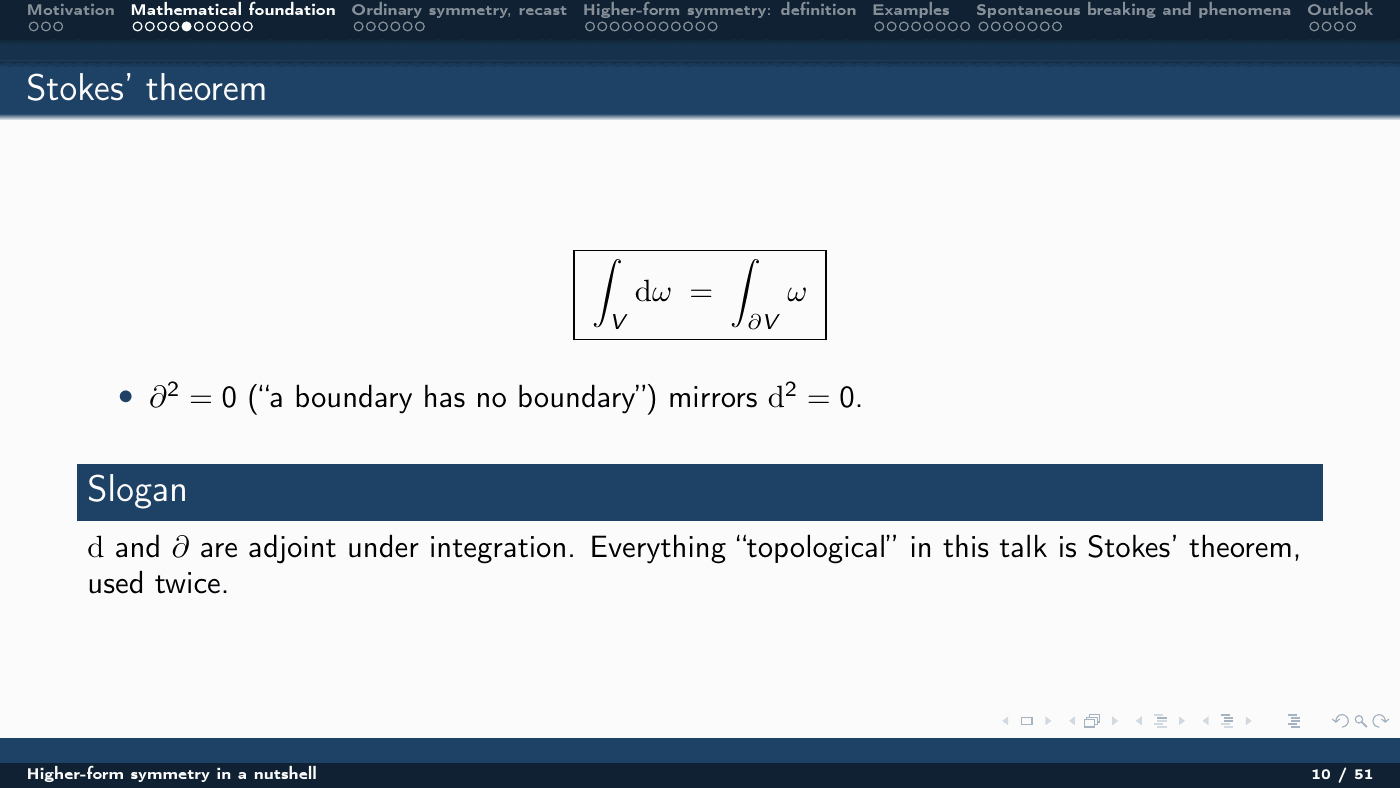
Stokes’ theorem $\int_V \mathrm{d}\omega = \int_{\partial V}\omega$, together with $\partial^2 = 0$ (“a boundary has no boundary”) mirroring $\mathrm{d}^2 = 0$, is the whole engine. The slogan from the slides: $\mathrm{d}$ and $\partial$ are adjoint under integration, and everything “topological” in this talk is Stokes’ theorem used twice.

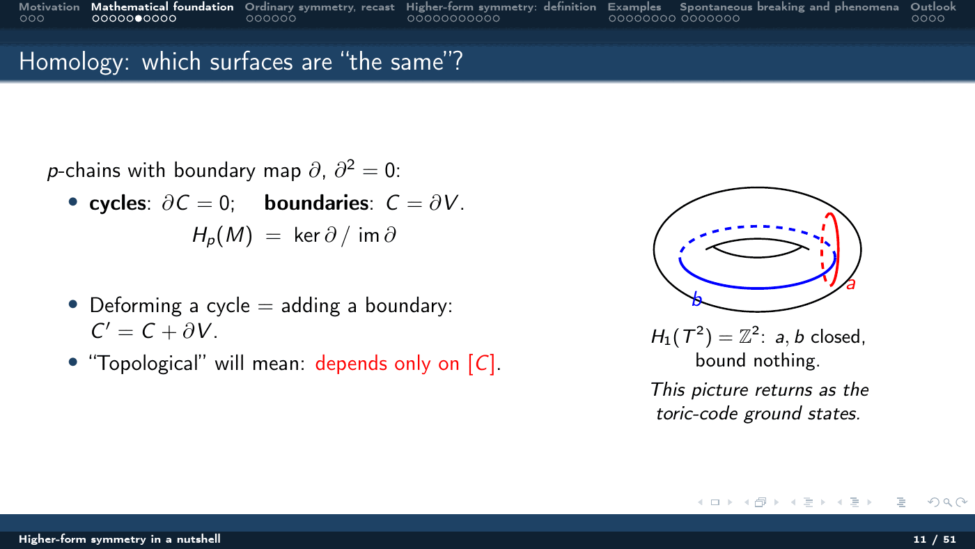
Homology asks which surfaces count as the same. With $p$-chains and the boundary map $\partial$, cycles are $\partial C = 0$ and boundaries are $C = \partial V$, so $H_p(M) = \ker\partial/\operatorname{im}\partial$. Deforming a cycle means adding a boundary, $C' = C + \partial V$, and “topological” will mean: depends only on the class $[C]$. The standing example is $H_1(T^2) = \mathbb{Z}^2$, the two cycles $a$ and $b$ that are closed but bound nothing — the same picture that later produces the toric code’s ground states.

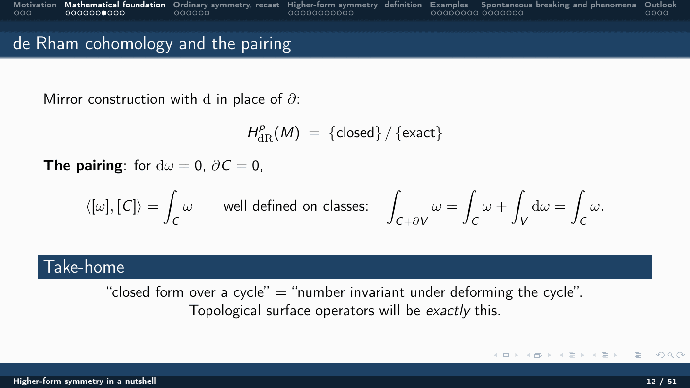
de Rham cohomology is the mirror construction with $\mathrm{d}$ in place of $\partial$: $H^p_{\mathrm{dR}}(M) = \{\text{closed}\}/\{\text{exact}\}$. The pairing is what matters. For $\mathrm{d}\omega = 0$ and $\partial C = 0$,

$$ \langle[\omega],[C]\rangle = \int_C \omega, \qquad \int_{C+\partial V}\omega = \int_C \omega + \int_V \mathrm{d}\omega = \int_C\omega, $$

so it is well defined on classes. Take-home: “closed form over a cycle” $=$ “number invariant under deforming the cycle” — and topological surface operators will be exactly this.

Poincaré duality and linking

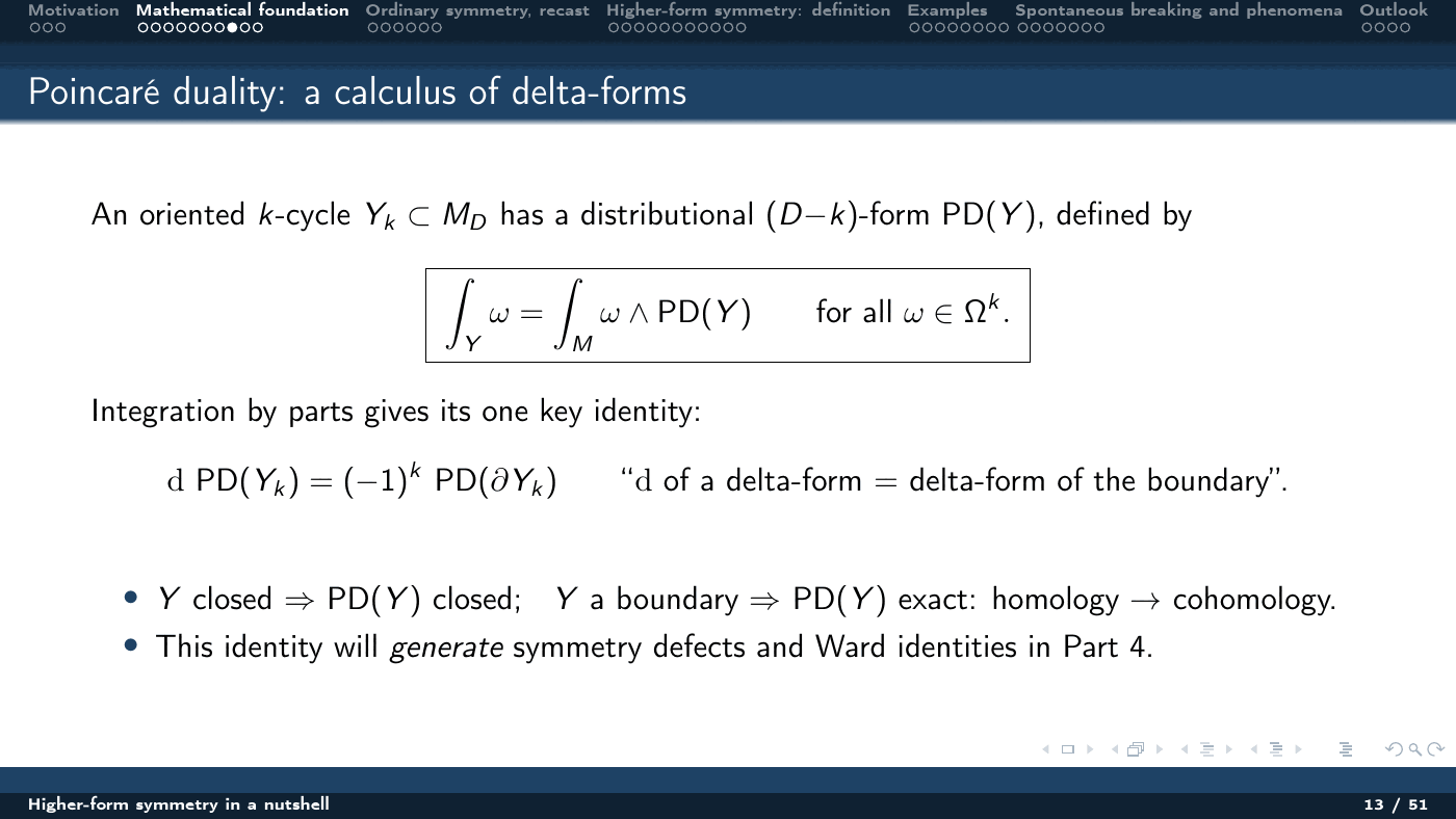
An oriented $k$-cycle $Y_k\subset M_D$ has a distributional $(D-k)$-form $\mathrm{PD}(Y)$ defined by $\int_Y \omega = \int_M \omega\wedge \mathrm{PD}(Y)$ for all $\omega\in\Omega^k$. Integration by parts gives its one key identity,

$$ \mathrm{d}\,\mathrm{PD}(Y_k) = (-1)^k\,\mathrm{PD}(\partial Y_k), $$

i.e. "$\mathrm{d}$ of a delta-form $=$ delta-form of the boundary." So $Y$ closed $\Rightarrow$ $\mathrm{PD}(Y)$ closed, and $Y$ a boundary $\Rightarrow$ $\mathrm{PD}(Y)$ exact: homology maps into cohomology. This identity is what generates symmetry defects and Ward identities later.

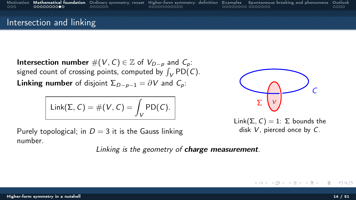
Finally, the intersection number $\#(V,C)\in\mathbb{Z}$ of $V_{D-p}$ with $C_p$ is the signed count of crossings, computed as $\int_V \mathrm{PD}(C)$; and for a disjoint $\Sigma_{D-p-1} = \partial V$,

$$ \mathrm{Link}(\Sigma,C) = \#(V,C) = \int_V \mathrm{PD}(C), $$

purely topological, and in $D=3$ the Gauss linking number. Linking is the geometry of charge measurement.

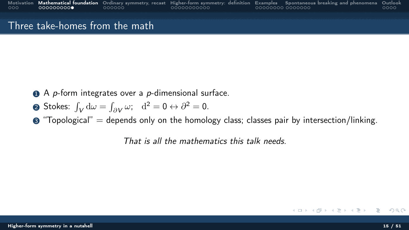
That is all the mathematics the talk needs, and it compresses to three take-homes: a $p$-form integrates over a $p$-dimensional surface; Stokes relates $\mathrm{d}$ and $\partial$; and “topological” means depending only on the homology class, with classes paired by intersection/linking.

Part 3 — Ordinary symmetry, recast

Noether in the language of forms

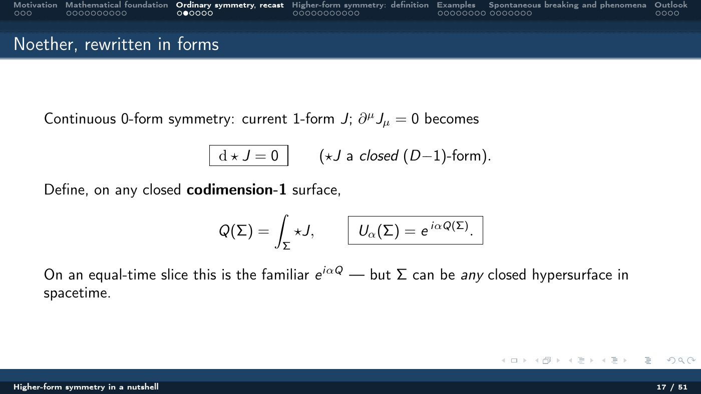
A continuous $0$-form symmetry has a current 1-form $J$, and $\partial^\mu J_\mu = 0$ becomes $\mathrm{d}\star J = 0$, i.e. $\star J$ is a closed $(D-1)$-form. On any closed codimension-1 surface define

$$ Q(\Sigma) = \int_\Sigma \star J,\qquad U_\alpha(\Sigma) = e^{i\alpha Q(\Sigma)} . $$

On an equal-time slice this is the familiar $e^{i\alpha Q}$ — but $\Sigma$ may be any closed hypersurface in spacetime.

The defect from a singular gauge parameter

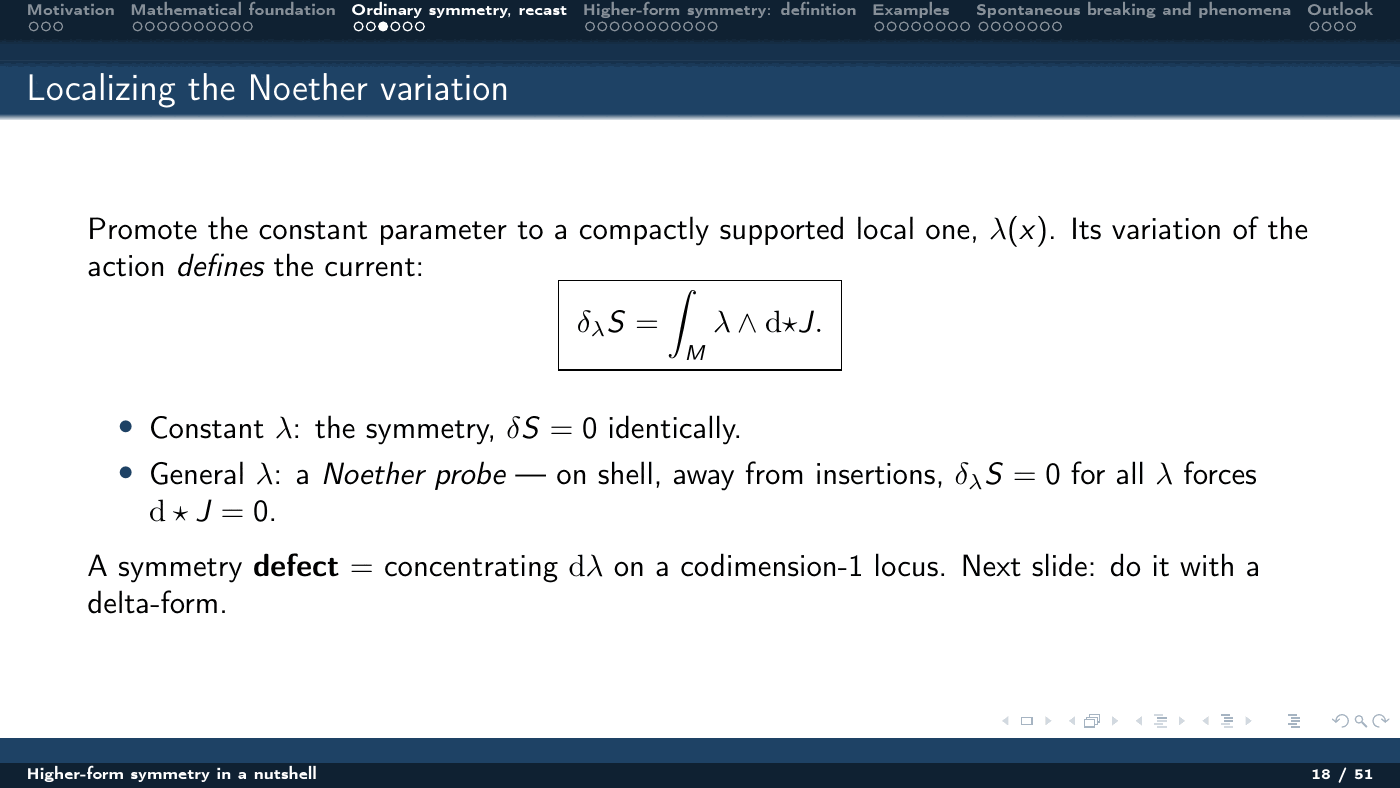
Promote the constant parameter to a compactly supported local one $\lambda(x)$; its variation of the action defines the current,

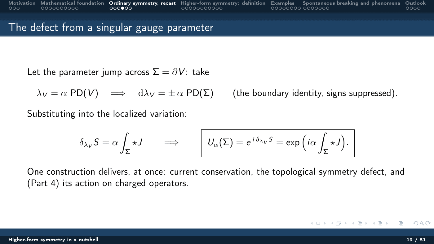
$$ \delta_\lambda S = \int_M \lambda\wedge \mathrm{d}\star J . $$

Constant $\lambda$ gives $\delta S = 0$ identically — the symmetry. General $\lambda$ is a Noether probe: on shell and away from insertions, $\delta_\lambda S = 0$ for all $\lambda$ forces $\mathrm{d}\star J = 0$. A symmetry defect is then just this variation with $\mathrm{d}\lambda$ concentrated on a codimension-1 locus. Taking $\Sigma = \partial V$ and $\lambda_V = \alpha\,\mathrm{PD}(V)$, the boundary identity gives $\mathrm{d}\lambda_V = \pm\alpha\,\mathrm{PD}(\Sigma)$ and hence

$$ \delta_{\lambda_V} S = \alpha\int_\Sigma \star J \qquad\Longrightarrow\qquad U_\alpha(\Sigma) = e^{\,i\delta_{\lambda_V}S} = \exp\!\Big(i\alpha\int_\Sigma \star J\Big). $$

One construction delivers three things at once: current conservation, the topological symmetry defect, and its action on charged operators.

Conservation is topological invariance

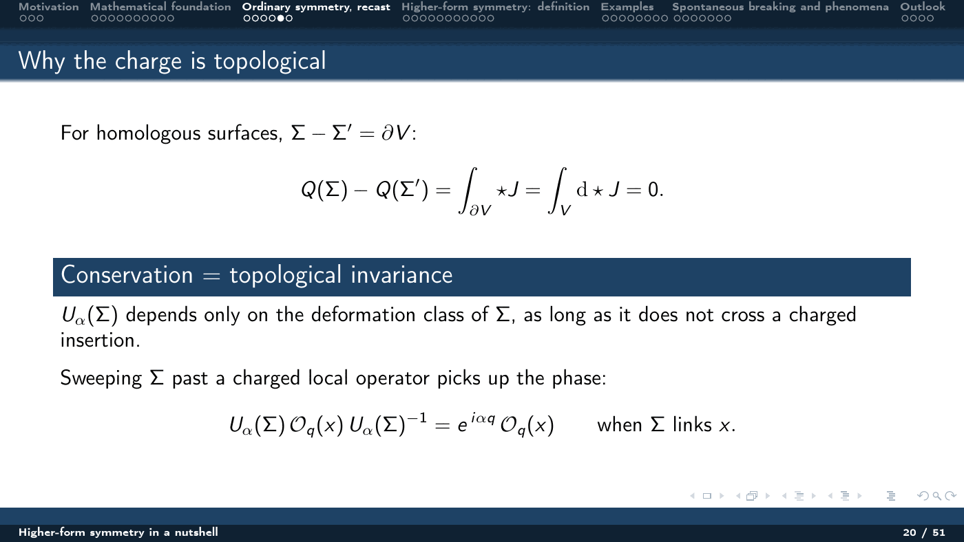
For homologous surfaces $\Sigma - \Sigma' = \partial V$,

$$ Q(\Sigma) - Q(\Sigma') = \int_{\partial V}\star J = \int_V \mathrm{d}\star J = 0 . $$

So $U_\alpha(\Sigma)$ depends only on the deformation class of $\Sigma$, as long as it does not cross a charged insertion — and sweeping $\Sigma$ past a charged local operator picks up the phase

$$ U_\alpha(\Sigma)\,\mathcal{O}_q(x)\,U_\alpha(\Sigma)^{-1} = e^{i\alpha q}\,\mathcal{O}_q(x) \qquad\text{when }\Sigma\text{ links }x . $$

The pivot

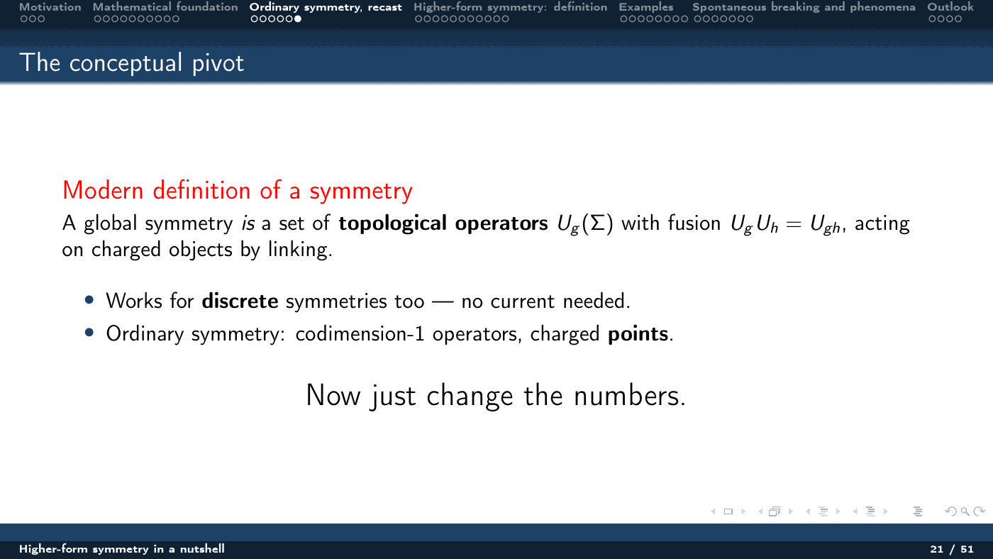
Modern definition of a symmetry. A global symmetry is a set of topological operators $U_g(\Sigma)$ with fusion $U_g U_h = U_{gh}$, acting on charged objects by linking.

This works for discrete symmetries too — no current is needed. Ordinary symmetry is the case of codimension-1 operators and charged points. Now just change the numbers.

Part 4 — Higher-form symmetry: the definition

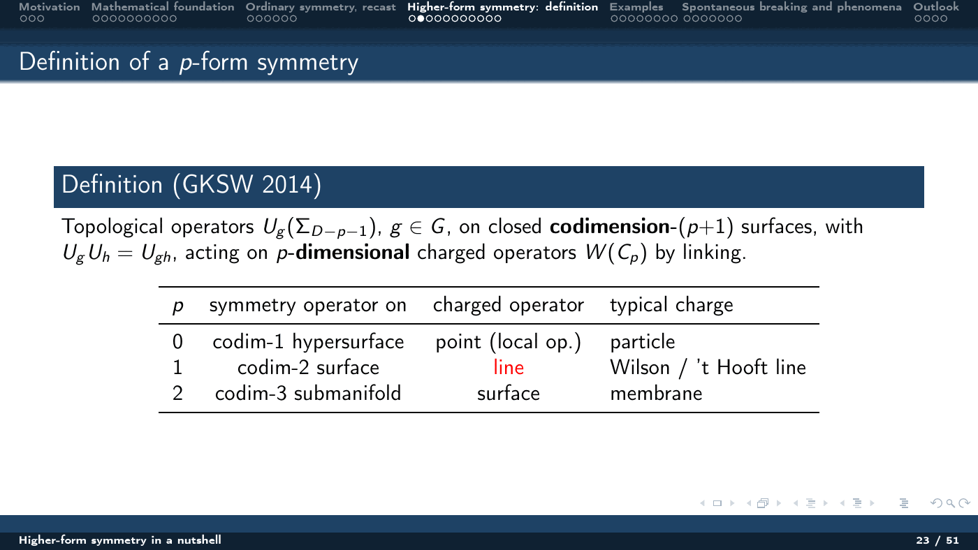
Definition (Gaiotto–Kapustin–Seiberg–Willett, 2014). Topological operators $U_g(\Sigma_{D-p-1})$, $g\in G$, on closed codimension-$(p+1)$ surfaces, with $U_g U_h = U_{gh}$, acting on $p$-dimensional charged operators $W(C_p)$ by linking.

$p$	symmetry operator on	charged operator	typical charge
0	codimension-1 hypersurface	point (local operator)	particle
1	codimension-2 surface	line	Wilson / ’t Hooft line
2	codimension-3 submanifold	surface	membrane

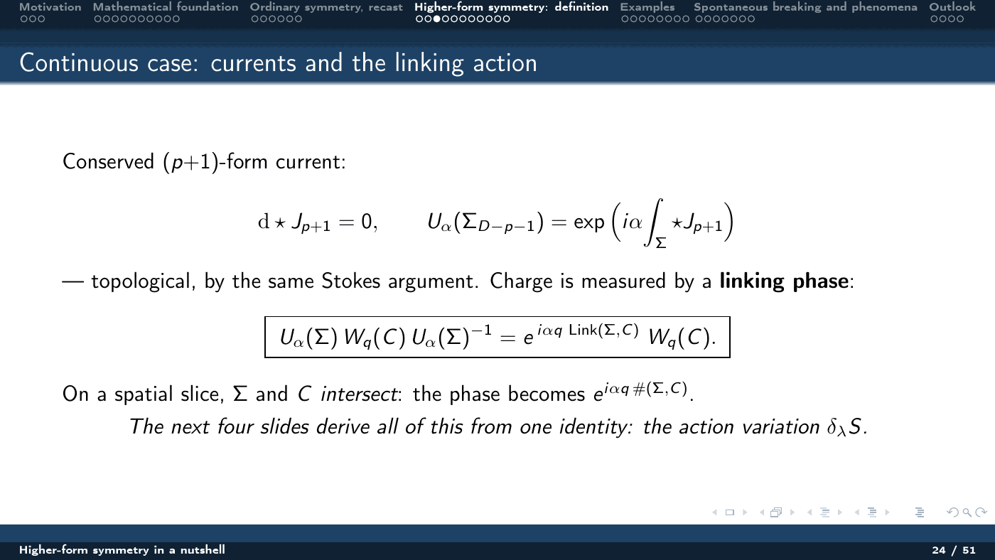
In the continuous case the conserved object is a $(p+1)$-form current,

$$ \mathrm{d}\star J_{p+1} = 0,\qquad U_\alpha(\Sigma_{D-p-1}) = \exp\!\Big(i\alpha\int_\Sigma \star J_{p+1}\Big), $$

topological by the same Stokes argument, with charge measured by a linking phase

$$ U_\alpha(\Sigma)\,W_q(C)\,U_\alpha(\Sigma)^{-1} = e^{\,i\alpha q\,\mathrm{Link}(\Sigma,C)}\,W_q(C). $$

On a spatial slice $\Sigma$ and $C$ intersect and the phase becomes $e^{i\alpha q\,\#(\Sigma,C)}$.

Everything from one identity

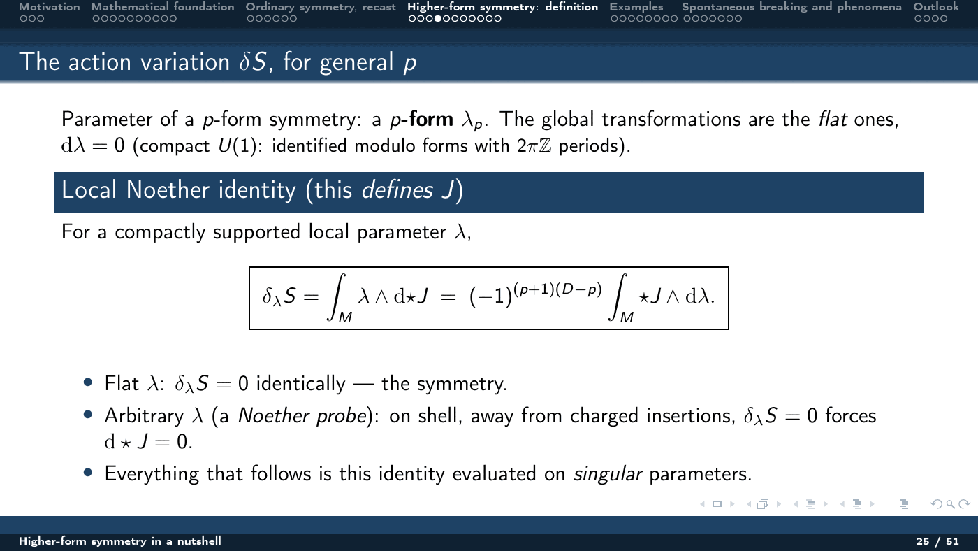
The parameter of a $p$-form symmetry is a $p$-form $\lambda_p$; the global transformations are the flat ones, $\mathrm{d}\lambda = 0$ (for compact $U(1)$, identified modulo forms with $2\pi\mathbb{Z}$ periods). The local Noether identity defines $J$:

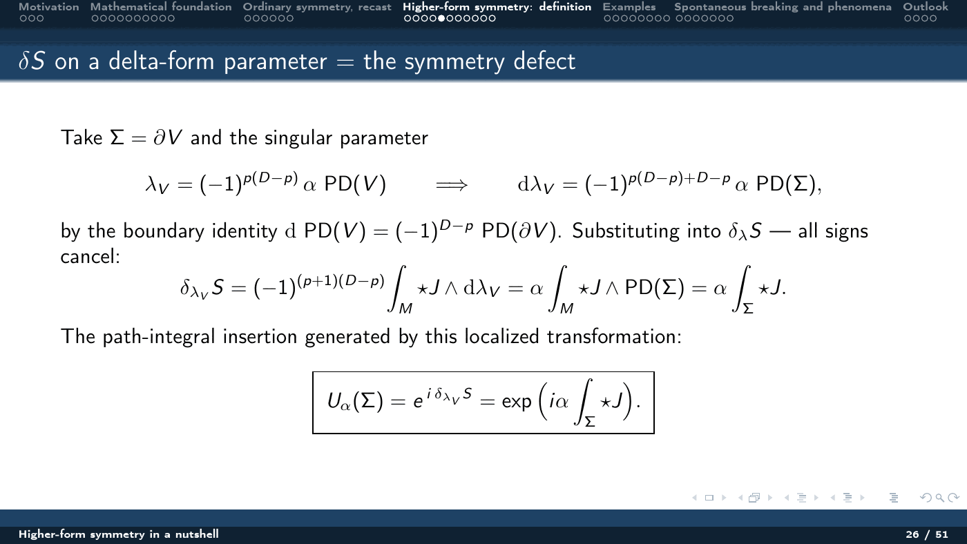
$$ \delta_\lambda S = \int_M \lambda\wedge\mathrm{d}\star J = (-1)^{(p+1)(D-p)}\int_M \star J\wedge \mathrm{d}\lambda . $$

Flat $\lambda$: $\delta_\lambda S = 0$ identically, the symmetry. Arbitrary $\lambda$: on shell and away from charged insertions, $\delta_\lambda S = 0$ forces $\mathrm{d}\star J = 0$. Evaluating it on the singular parameter $\lambda_V = (-1)^{p(D-p)}\alpha\,\mathrm{PD}(V)$, with $\mathrm{d}\,\mathrm{PD}(V) = (-1)^{D-p}\mathrm{PD}(\partial V)$, all signs cancel and

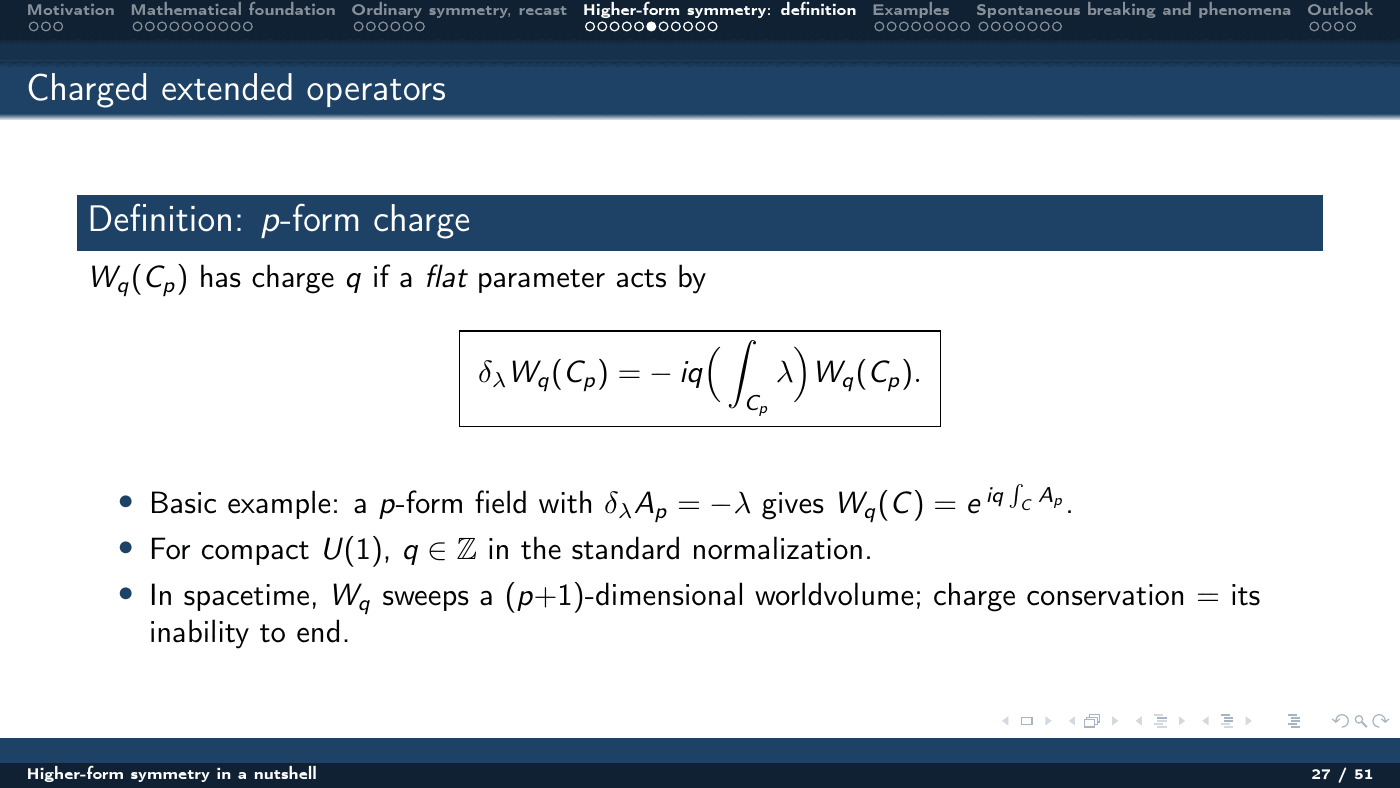
$$ \delta_{\lambda_V}S = \alpha\int_M \star J\wedge \mathrm{PD}(\Sigma) = \alpha\int_\Sigma \star J \qquad\Longrightarrow\qquad U_\alpha(\Sigma) = \exp\!\Big(i\alpha\int_\Sigma \star J\Big). $$

A charged operator $W_q(C_p)$ is one on which a flat parameter acts by $\delta_\lambda W_q(C_p) = -iq\big(\int_{C_p}\lambda\big)W_q(C_p)$; the basic example is a $p$-form field with $\delta_\lambda A_p = -\lambda$, giving $W_q(C) = e^{\,iq\oint_C A_p}$, with $q\in\mathbb{Z}$ for compact $U(1)$. In spacetime $W_q$ sweeps a $(p+1)$-dimensional worldvolume, and charge conservation is its inability to end.

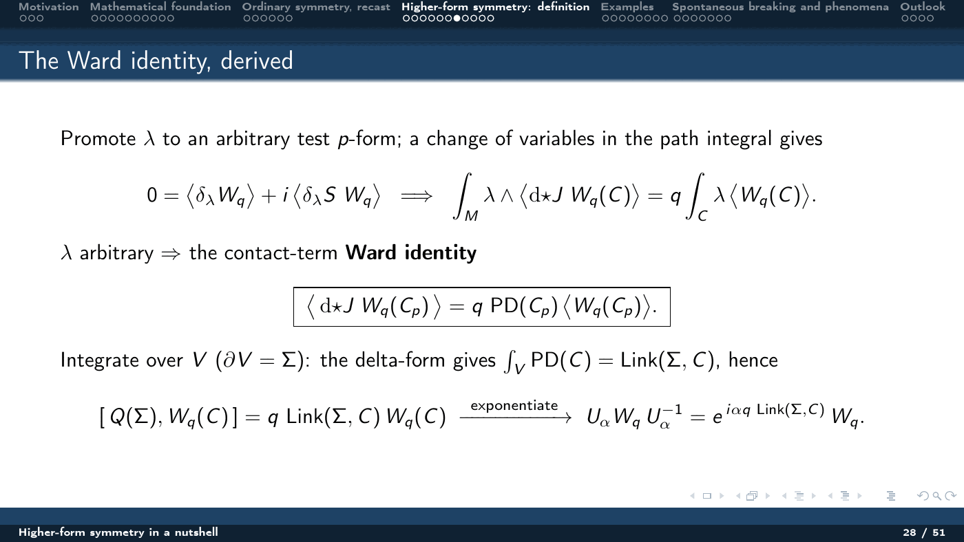
Promoting $\lambda$ to an arbitrary test $p$-form and changing variables in the path integral,

$$ 0 = \langle\delta_\lambda W_q\rangle + i\langle \delta_\lambda S\, W_q\rangle \quad\Longrightarrow\quad \mathrm{d}\star J\, W_q(C_p) = q\,\mathrm{PD}(C_p)\,W_q(C_p), $$

the contact-term Ward identity. Integrating over $V$ with $\partial V = \Sigma$, the delta-form gives $\int_V \mathrm{PD}(C) = \mathrm{Link}(\Sigma,C)$, hence

$$ [\,Q(\Sigma), W_q(C)\,] = q\,\mathrm{Link}(\Sigma,C)\,W_q(C) \;\xrightarrow{\ \text{exponentiate}\ }\; U_\alpha W_q U_\alpha^{-1} = e^{\,i\alpha q\,\mathrm{Link}(\Sigma,C)}W_q . $$

Higher-form symmetries are abelian

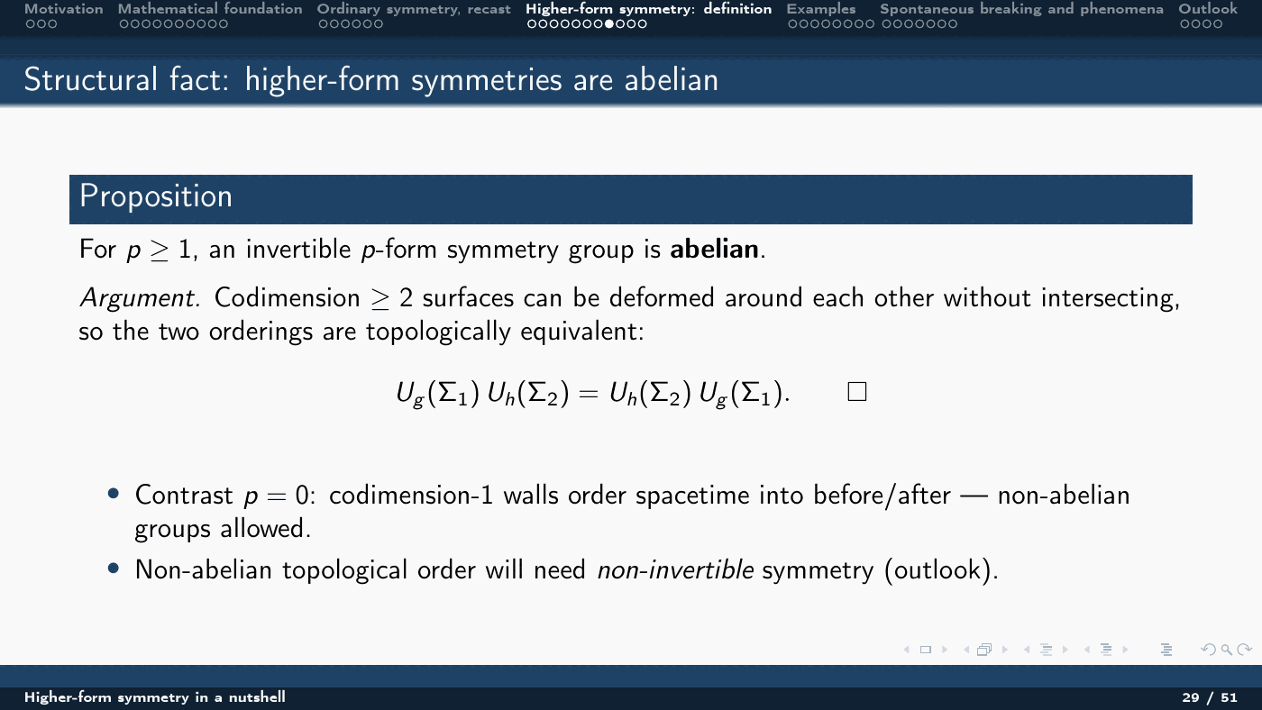
Proposition. For $p\ge 1$, an invertible $p$-form symmetry group is abelian.

The argument is one line of topology: surfaces of codimension $\ge 2$ can be deformed around each other without intersecting, so the two orderings are topologically equivalent, $U_g(\Sigma_1)U_h(\Sigma_2) = U_h(\Sigma_2)U_g(\Sigma_1)$. Contrast $p=0$, where codimension-1 walls order spacetime into before/after and non-abelian groups are allowed. Non-abelian topological order will therefore require non-invertible symmetry — see the outlook.

Background fields and gauging

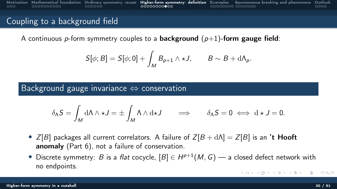
A continuous $p$-form symmetry couples to a background $(p+1)$-form gauge field,

$$ S[\phi;B] = S[\phi;0] + \int_M B_{p+1}\wedge\star J, \qquad B\sim B + \mathrm{d}\Lambda_p, $$

and background gauge invariance is conservation: $\delta_\Lambda S = \int_M \mathrm{d}\Lambda\wedge\star J = \pm\int_M \Lambda\wedge \mathrm{d}\star J$, so $\delta_\Lambda S = 0 \Leftrightarrow \mathrm{d}\star J = 0$. The partition function $Z[B]$ packages all current correlators, and a failure of $Z[B+\mathrm{d}\Lambda] = Z[B]$ is an ’t Hooft anomaly, not a failure of conservation. For a discrete symmetry $B$ is a flat cocycle, $[B]\in H^{p+1}(M,G)$ — a closed defect network with no endpoints.

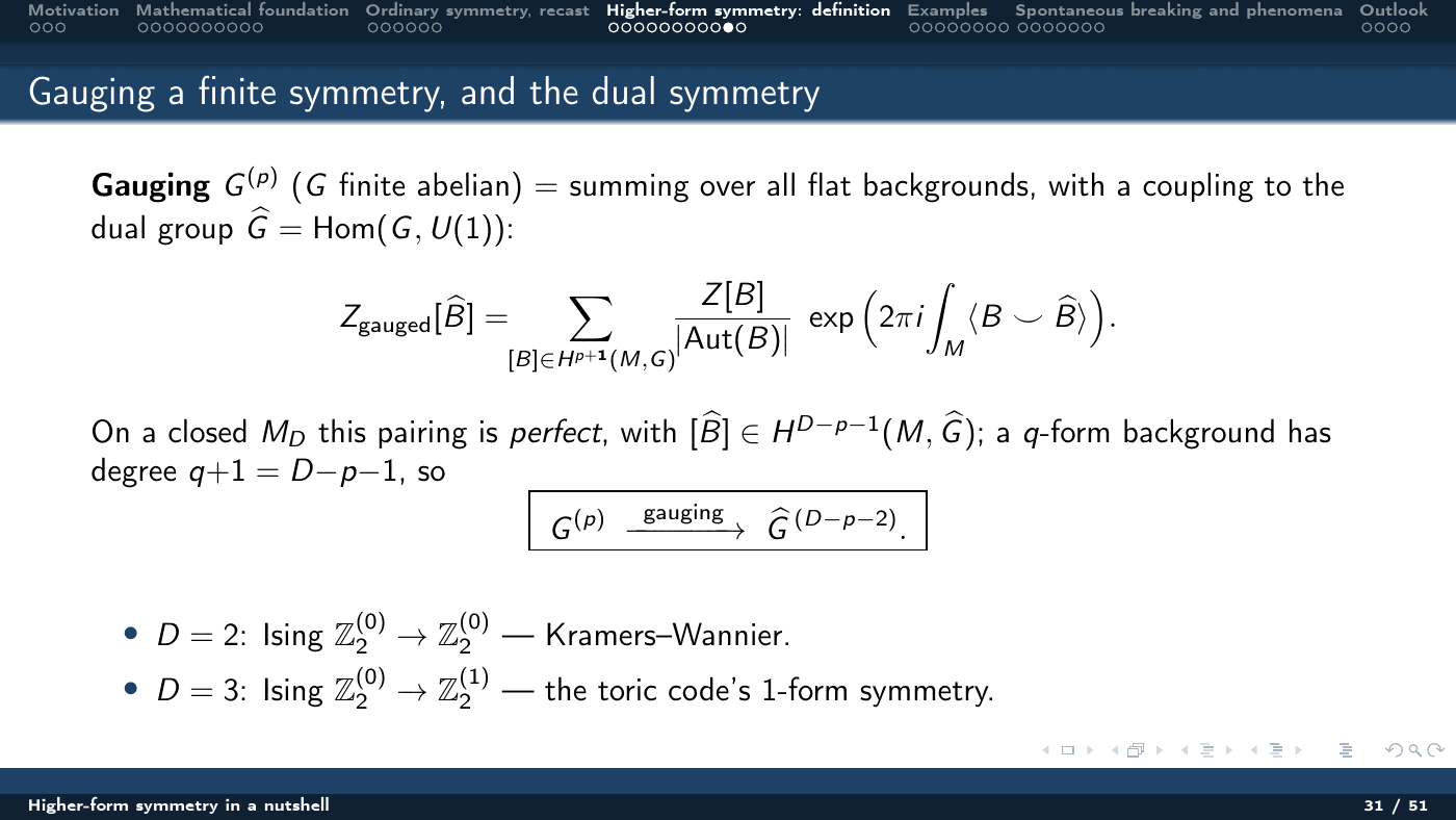
Gauging a finite abelian $G^{(p)}$ means summing over flat backgrounds while coupling to the dual group $\hat G = \operatorname{Hom}(G,U(1))$:

$$ Z_{\text{gauged}}[\hat B] = \sum_{[B]\in H^{p+1}(M,G)}\frac{Z[B]}{|\mathrm{Aut}(B)|} \exp\!\Big(2\pi i \int_M \langle B\smile \hat B\rangle\Big). $$

On a closed $M_D$ the pairing is perfect with $[\hat B]\in H^{D-p-1}(M,\hat G)$, and since a $q$-form background has degree $q+1 = D-p-1$,

$$ G^{(p)} \;\xrightarrow{\ \text{gauging}\ }\; \hat G^{(D-p-2)} . $$

In $D=2$ this is Ising $\mathbb{Z}_2^{(0)}\to\mathbb{Z}_2^{(0)}$ — Kramers–Wannier. In $D=3$ it is $\mathbb{Z}_2^{(0)}\to\mathbb{Z}_2^{(1)}$ — the toric code’s 1-form symmetry.

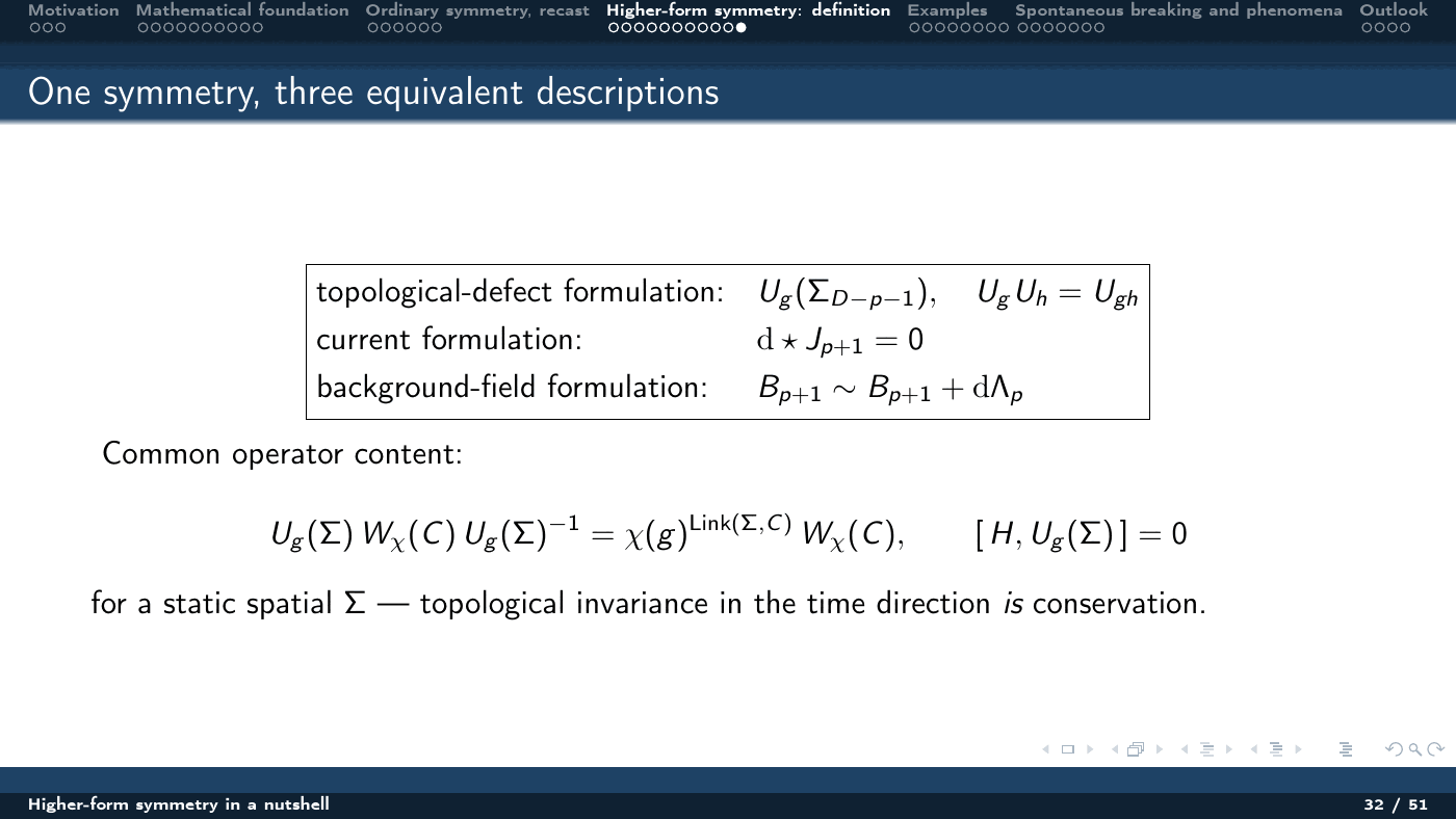
The upshot is that one symmetry admits three equivalent descriptions — topological defects $U_g(\Sigma_{D-p-1})$ with $U_gU_h = U_{gh}$; a current with $\mathrm{d}\star J_{p+1} = 0$; and a background field with $B_{p+1}\sim B_{p+1}+\mathrm{d}\Lambda_p$ — sharing the operator content $U_g(\Sigma)W_\chi(C)U_g(\Sigma)^{-1} = \chi(g)^{\mathrm{Link}(\Sigma,C)}W_\chi(C)$ and $[H,U_g(\Sigma)] = 0$ for static spatial $\Sigma$, where topological invariance in the time direction is conservation.

Part 5 — Examples

Maxwell in $D=4$: two 1-form symmetries

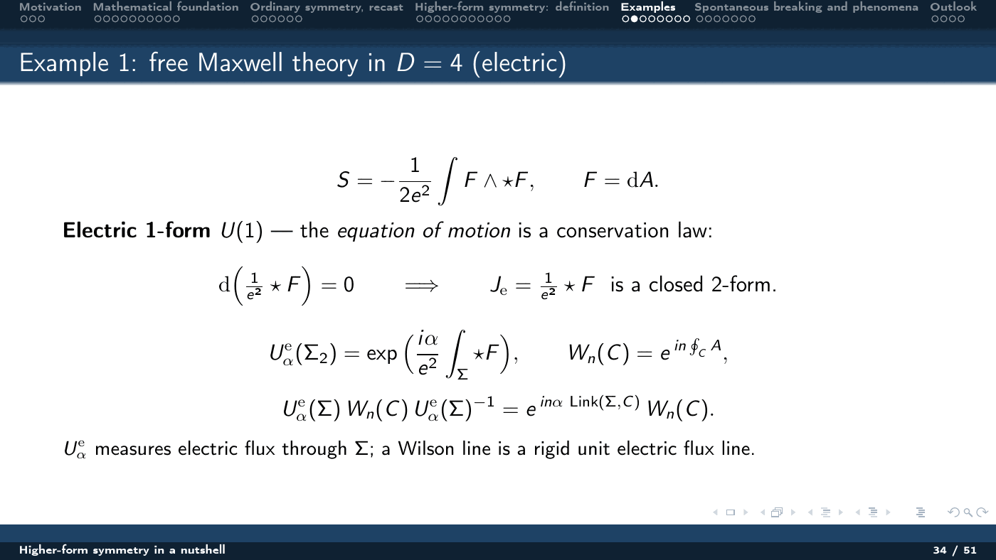
From $S = -\frac{1}{2e^2}\int F\wedge\star F$ with $F = \mathrm{d}A$, the equation of motion $\mathrm{d}\big(\tfrac{1}{e^2}\star F\big) = 0$ is a conservation law: $J_e = \tfrac{1}{e^2}\star F$ is a closed 2-form, giving an electric $U(1)$ 1-form symmetry

$$ U^e_\alpha(\Sigma_2) = \exp\!\Big(\frac{i\alpha}{e^2}\int_\Sigma \star F\Big), \qquad W_n(C) = e^{\,in\oint_C A}, $$

with $U^e_\alpha(\Sigma)W_n(C)U^e_\alpha(\Sigma)^{-1} = e^{\,in\alpha\,\mathrm{Link}(\Sigma,C)} W_n(C)$. So $U^e_\alpha$ measures electric flux through $\Sigma$, and a Wilson line is a rigid unit electric flux line.

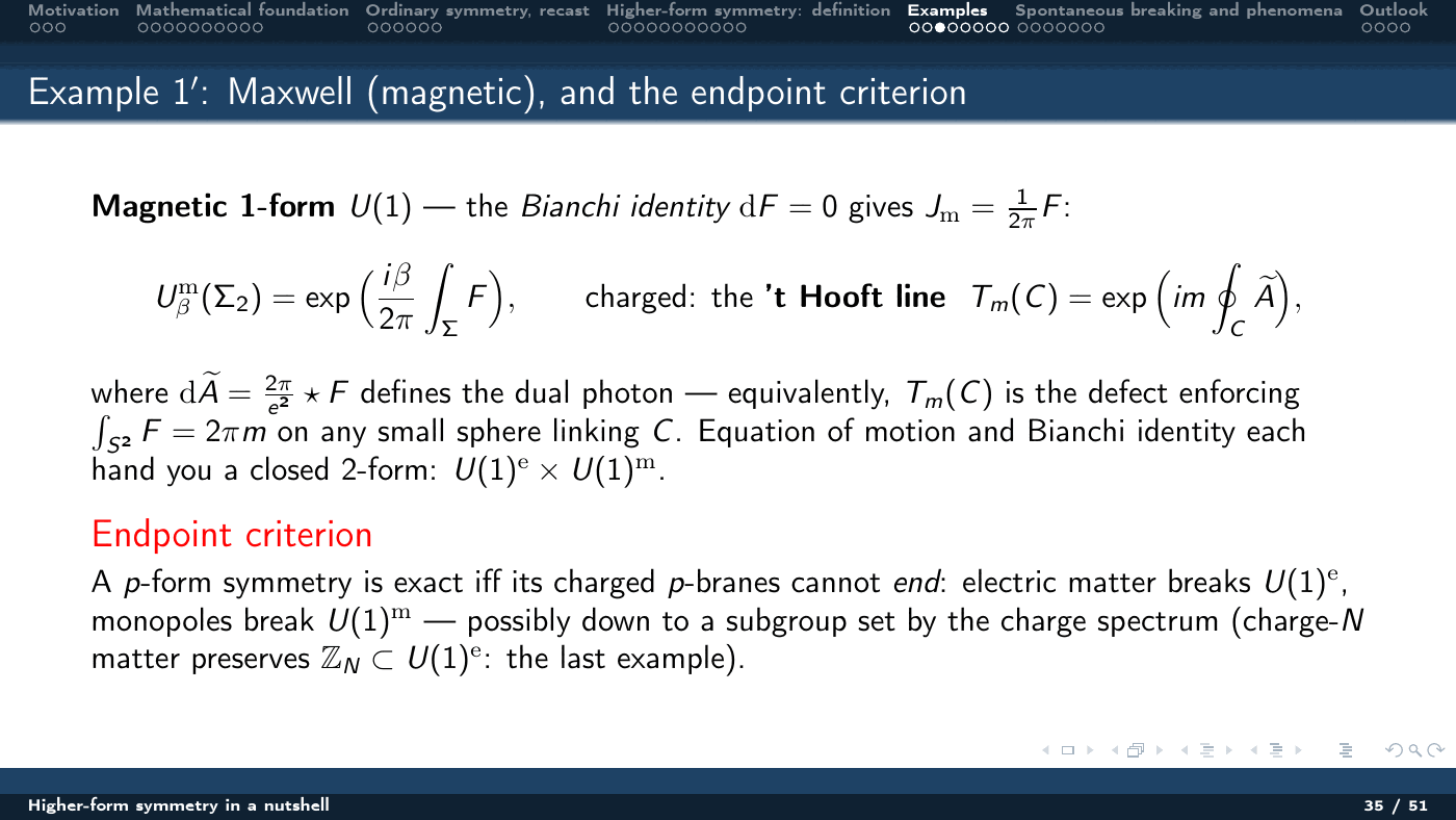
The Bianchi identity $\mathrm{d}F = 0$ hands over a second closed 2-form, $J_m = \tfrac{1}{2\pi}F$, i.e. a magnetic 1-form symmetry $U^m_\beta(\Sigma_2) = \exp\big(\tfrac{i\beta}{2\pi}\int_\Sigma F\big)$, whose charged object is the ’t Hooft line $T_m(C) = \exp\big(im\oint_C A_e\big)$ with $\mathrm{d}A_e = \tfrac{2\pi}{e^2}\star F$ the dual photon — equivalently, the defect enforcing $\int_{S^2} F = 2\pi m$ on any small sphere linking $C$. Equation of motion and Bianchi identity each give a conserved 2-form current: $U(1)_e\times U(1)_m$.

Endpoint criterion. A $p$-form symmetry is exact iff its charged $p$-branes cannot end. Electric matter breaks $U(1)_e$ and monopoles break $U(1)_m$ — possibly only down to a subgroup set by the charge spectrum, since charge-$N$ matter preserves $\mathbb{Z}_N\subset U(1)_e$.

Toric code and $\mathbb{Z}_N$ gauge theory

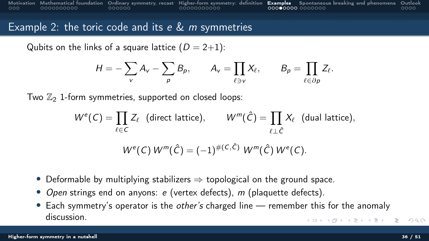
With qubits on the links of a square lattice in $D = 2+1$,

$$ H = -\sum_v A_v - \sum_p B_p,\qquad A_v = \prod_{\ell\ni v} X_\ell,\qquad B_p = \prod_{\ell\in\partial p} Z_\ell, $$

there are two $\mathbb{Z}_2$ 1-form symmetries supported on closed loops, $W^e(C) = \prod_{\ell\in C}Z_\ell$ on the direct lattice and $W^m(\hat C) = \prod_{\ell\perp\hat C}X_\ell$ on the dual lattice, obeying

$$ W^e(C)\,W^m(\hat C) = (-1)^{\#(C,\hat C)}\,W^m(\hat C)\,W^e(C). $$

They are deformable by multiplying stabilizers, hence topological on the ground space; open strings end on anyons ($e$ at vertex defects, $m$ at plaquette defects); and each symmetry’s operator is the other’s charged line — the fact that returns in the anomaly discussion.

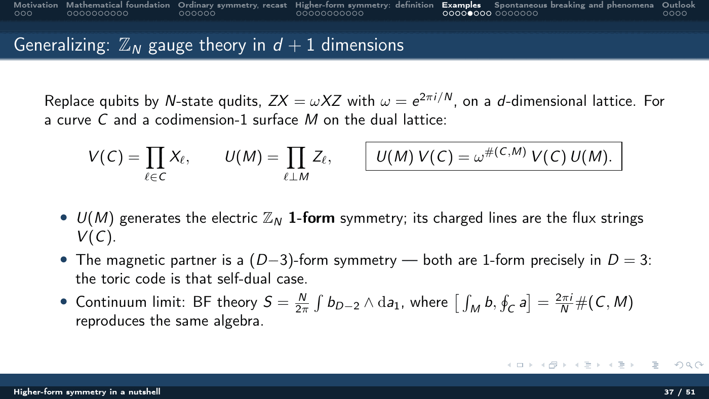
Generalizing to $N$-state qudits with $ZX = \omega XZ$, $\omega = e^{2\pi i/N}$, on a $d$-dimensional lattice, with $V(C) = \prod_{\ell\in C}X_\ell$ and $U(M) = \prod_{\ell\perp M}Z_\ell$ for a curve $C$ and a dual codimension-1 surface $M$,

$$ U(M)\,V(C) = \omega^{\#(C,M)}\,V(C)\,U(M). $$

$U(M)$ generates the electric $\mathbb{Z}_N$ 1-form symmetry and its charged lines are the flux strings $V(C)$; the magnetic partner is a $(D-3)$-form symmetry, so both are 1-form precisely in $D=3$ — the toric code is that self-dual case. The continuum limit is BF theory $S = \frac{N}{2\pi}\int b_{D-2}\wedge \mathrm{d}a_1$, where $\big\langle \int_M b,\oint_C a\big\rangle = \frac{2\pi i}{N}\#(C,M)$ reproduces the same algebra.

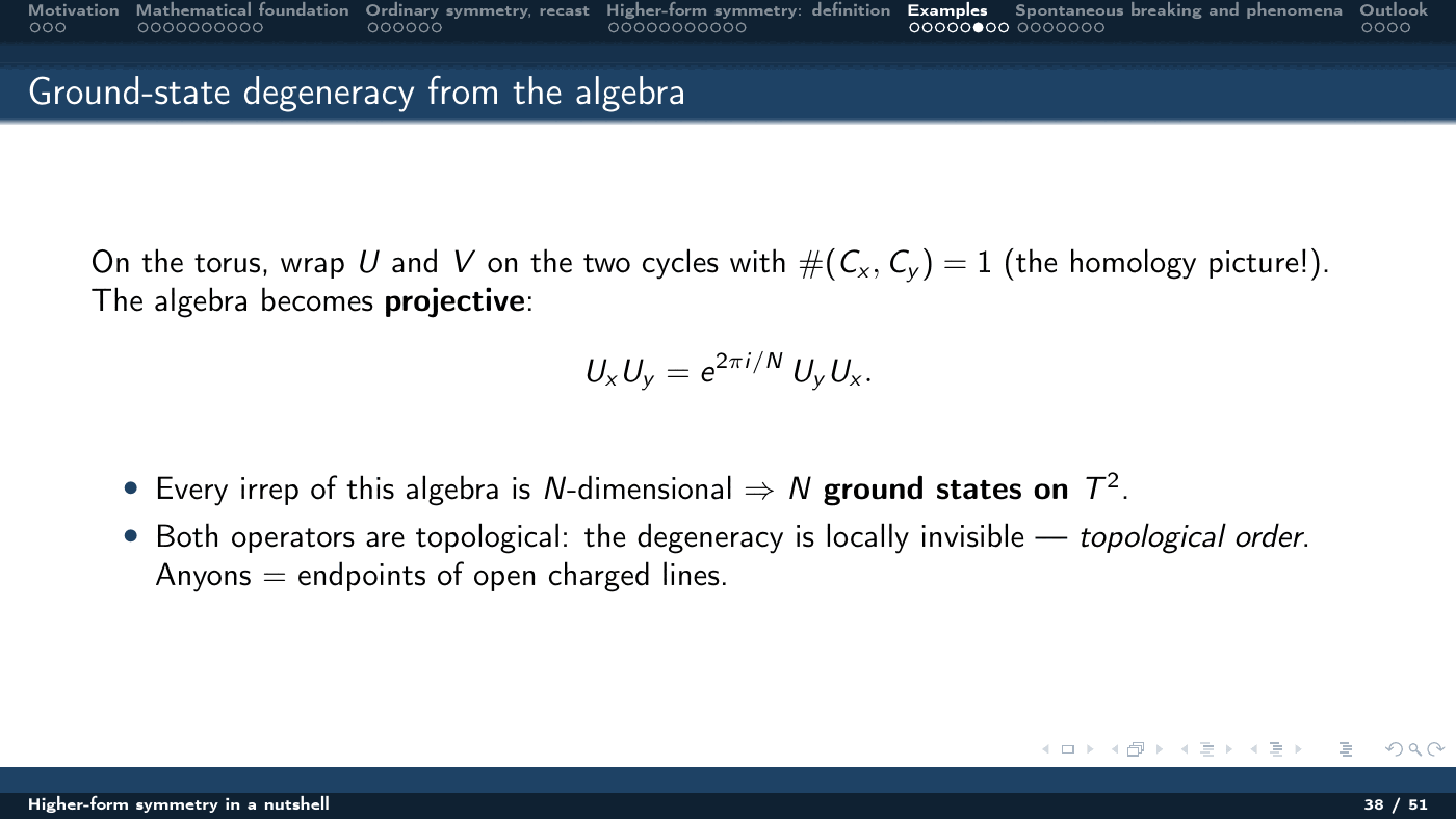
Wrapping $U$ and $V$ on the two cycles of a torus with $\#(C_x,C_y) = 1$ — the homology picture from Part 2 — makes the algebra projective,

$$ U_x U_y = e^{2\pi i/N}\,U_y U_x, $$

every irrep of which is $N$-dimensional, so there are $N$ ground states on $T^2$. Both operators are topological, so the degeneracy is locally invisible: topological order, with anyons as the endpoints of open charged lines.

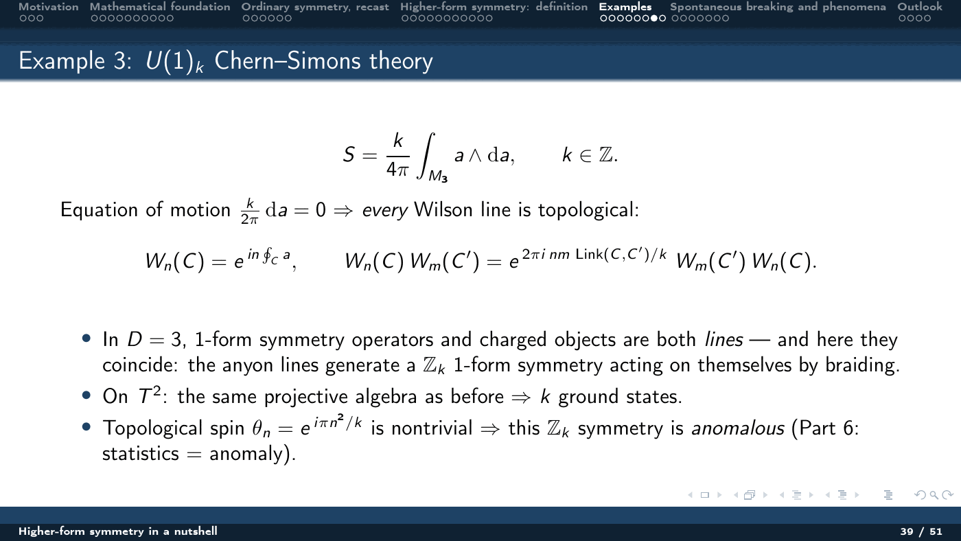
$U(1)_k$ Chern–Simons

For $S = \frac{k}{4\pi}\int_{M_3} a\wedge \mathrm{d}a$ with $k\in\mathbb{Z}$, the equation of motion $\frac{k}{2\pi}\mathrm{d}a = 0$ makes every Wilson line topological, and

$$ W_n(C)\,W_m(C') = e^{\,2\pi i\,nm\,\mathrm{Link}(C,C')/k}\,W_m(C')\,W_n(C). $$

In $D=3$ the 1-form symmetry operators and the charged objects are both lines — and here they coincide: the anyon lines generate a $\mathbb{Z}_k$ 1-form symmetry acting on themselves by braiding. On $T^2$ the same projective algebra gives $k$ ground states. The topological spin $\theta_n = e^{i\pi n^2/k}$ is nontrivial, which makes this $\mathbb{Z}_k$ symmetry anomalous — statistics as anomaly, picked up again in Part 6.

$SU(N)$ center symmetry and confinement

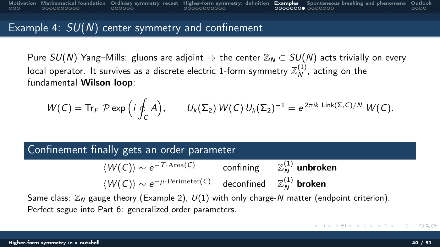
In pure $SU(N)$ Yang–Mills the gluons are adjoint, so the center $\mathbb{Z}_N\subset SU(N)$ acts trivially on every local operator. It survives as a discrete electric 1-form symmetry $\mathbb{Z}_N^{(1)}$ acting on the fundamental Wilson loop,

$$ U_k(\Sigma_2)\,W(C)\,U_k(\Sigma_2)^{-1} = e^{\,2\pi i k\,\mathrm{Link}(\Sigma,C)/N}\,W(C), \qquad W(C) = \mathrm{Tr}_F\,\mathcal{P}\exp\Big(i\oint_C A\Big). $$

This finally gives confinement an order parameter:

$\langle W(C)\rangle\sim e^{-T\cdot\mathrm{Area}(C)}$	confining — $\mathbb{Z}_N^{(1)}$ unbroken
$\langle W(C)\rangle\sim e^{-\mu\cdot\mathrm{Perimeter}(C)}$	deconfined — $\mathbb{Z}_N^{(1)}$ broken

$\mathbb{Z}_N$ gauge theory and $U(1)$ with only charge-$N$ matter sit in the same class, by the endpoint criterion.

Part 6 — Spontaneous breaking and its phenomena

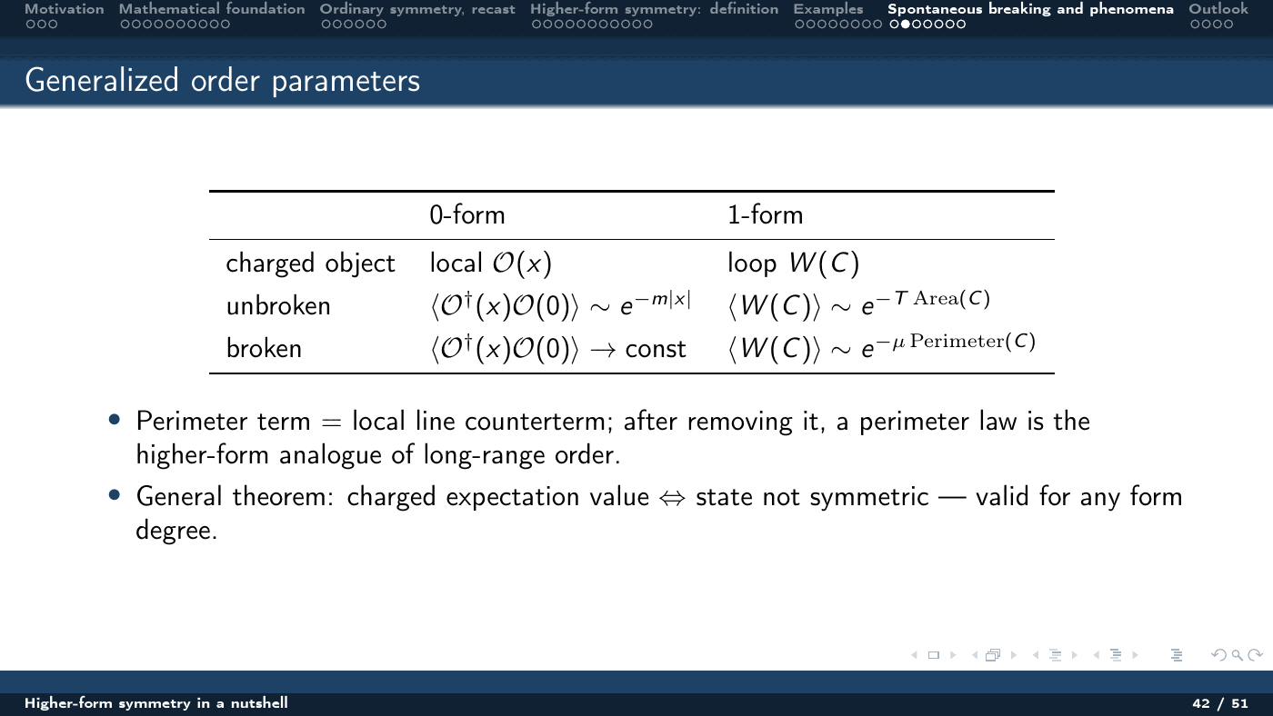
Generalized order parameters

	0-form	1-form
charged object	local $\mathcal{O}(x)$	loop $W(C)$
unbroken	$\langle\mathcal{O}^\dagger(x)\mathcal{O}(0)\rangle\sim e^{-m\lvert x\rvert}$	$\langle W(C)\rangle\sim e^{-T\,\mathrm{Area}(C)}$
broken	$\langle\mathcal{O}^\dagger(x)\mathcal{O}(0)\rangle\to\text{const}$	$\langle W(C)\rangle\sim e^{-\mu\,\mathrm{Perimeter}(C)}$

The perimeter term is a local line counterterm; after removing it, a perimeter law is the higher-form analogue of long-range order. The general theorem — a nonzero charged expectation value means the state is not symmetric — holds at any form degree.

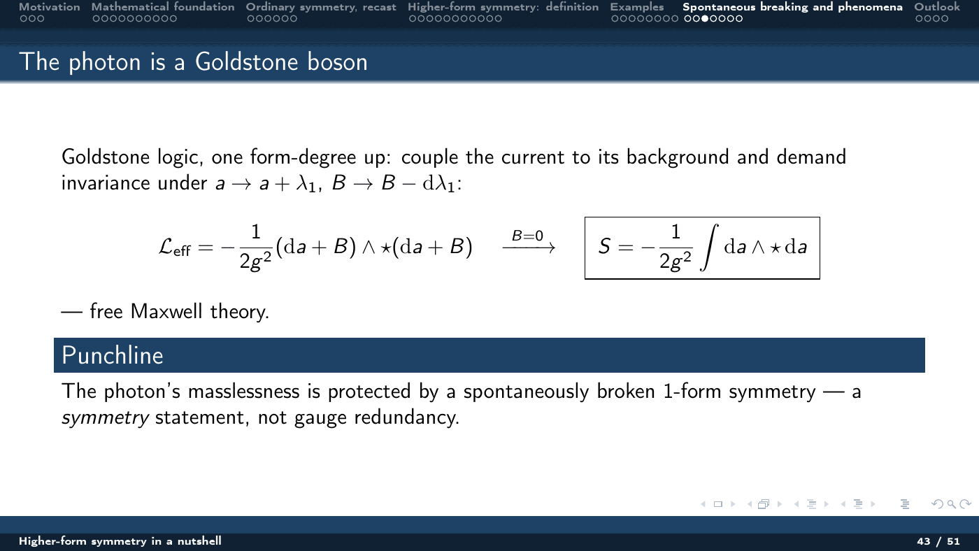
The photon is a Goldstone boson

Run the Goldstone logic one form-degree up: couple the current to its background and demand invariance under $a\to a+\lambda_1$, $B\to B-\mathrm{d}\lambda_1$,

$$ \mathcal{L}_{\text{eff}} = -\frac{1}{2g^2}(\mathrm{d}a+B)\wedge\star(\mathrm{d}a+B) \;\xrightarrow{\ B=0\ }\; S = -\frac{1}{2g^2}\int \mathrm{d}a\wedge\star \mathrm{d}a, $$

which is free Maxwell theory. The photon’s masslessness is protected by a spontaneously broken 1-form symmetry — a symmetry statement, not gauge redundancy.

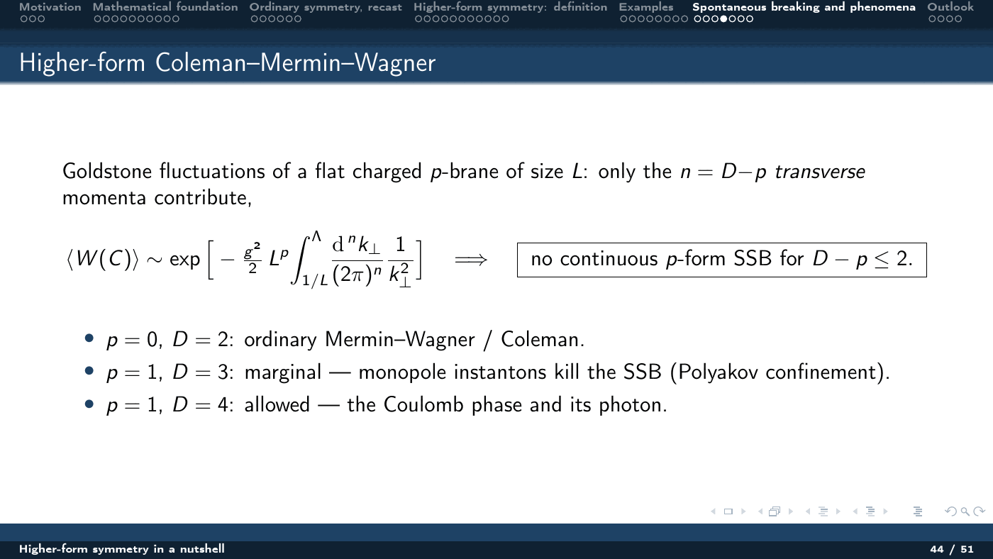
Higher-form Coleman–Mermin–Wagner

Estimate the Goldstone fluctuations of a flat charged $p$-brane of size $L$: only the $n = D-p$ transverse momenta contribute,

$$ \langle W(C)\rangle \sim \exp\Big[-\frac{g^2}{2}L^p\int_{1/L}^{\Lambda} \frac{\mathrm{d}^n k_\perp}{(2\pi)^n}\frac{1}{k_\perp^2}\Big] \quad\Longrightarrow\quad \text{no continuous $p$-form SSB for } D-p\le 2 . $$

At $p=0$, $D=2$ this is ordinary Mermin–Wagner/Coleman. At $p=1$, $D=3$ it is marginal, and monopole instantons kill the SSB — Polyakov confinement. At $p=1$, $D=4$ it is allowed: the Coulomb phase and its photon.

Topological order $=$ higher-form SSB… almost

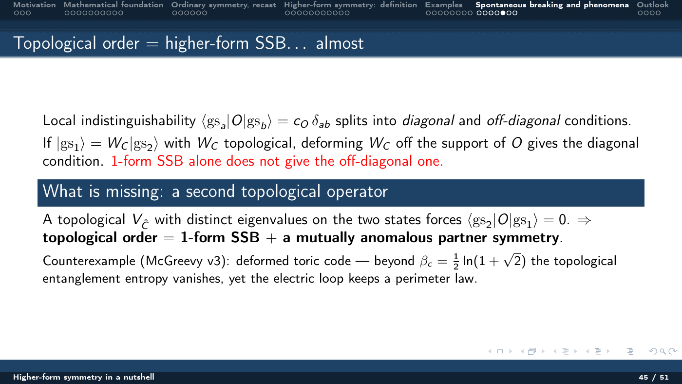
Local indistinguishability $\langle \mathrm{gs}_a|\mathcal{O}|\mathrm{gs}_b\rangle = c_{\mathcal{O}}\delta_{ab}$ splits into a diagonal and an off-diagonal condition. If $|\mathrm{gs}_1\rangle = W_C|\mathrm{gs}_2\rangle$ with $W_C$ topological, deforming $W_C$ off the support of $\mathcal{O}$ gives the diagonal condition — but 1-form SSB alone does not give the off-diagonal one.

What is missing is a second topological operator: a topological $V_{\hat C}$ with distinct eigenvalues on the two states forces $\langle \mathrm{gs}_2|\mathcal{O}|\mathrm{gs}_1\rangle = 0$. So topological order is 1-form SSB plus a mutually anomalous partner symmetry. McGreevy’s counterexample (v3) makes the point sharp: in the deformed toric code, beyond $\beta_c = \tfrac12\ln(1+\sqrt{2})$ the topological entanglement entropy vanishes while the electric loop still obeys a perimeter law.

’t Hooft anomalies

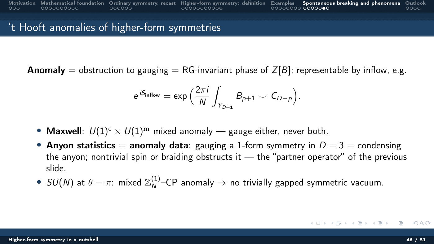
An anomaly is an obstruction to gauging — an RG-invariant phase of $Z[B]$, representable by inflow, e.g.

$$ e^{\,iS_{\text{inflow}}} = \exp\Big(\frac{2\pi i}{N}\int_{Y_{D+1}} B_{p+1}\smile C_{D-p}\Big). $$

Three instances from the talk: Maxwell has a mixed $U(1)_e\times U(1)_m$ anomaly, so you may gauge either but never both; anyon statistics are anomaly data, since gauging a 1-form symmetry in $D=3$ is condensing the anyon and nontrivial spin or braiding obstructs it — that is the “partner operator” of the previous slide; and $SU(N)$ at $\theta = \pi$ has a mixed $\mathbb{Z}_N^{(1)}$–$CP$ anomaly, forbidding a trivially gapped symmetric vacuum.

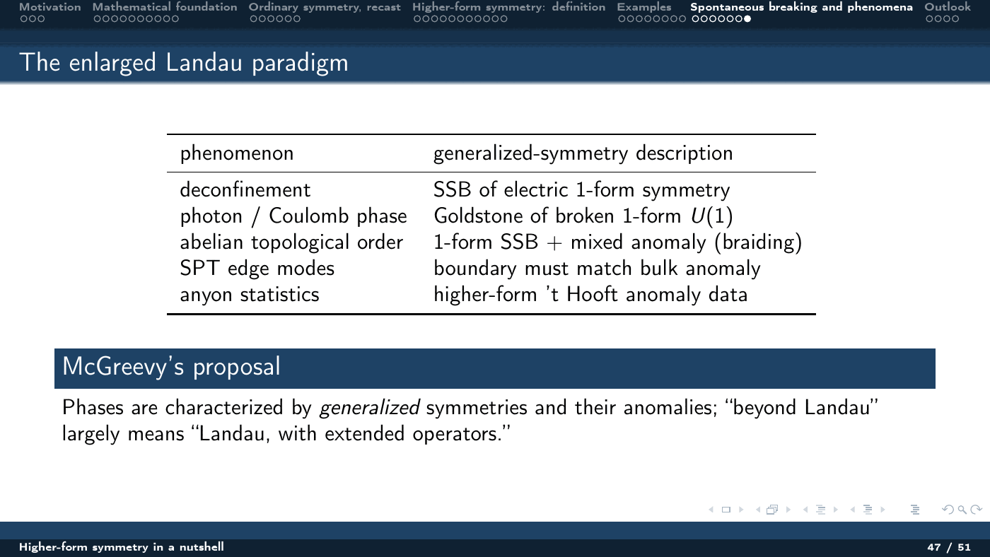
The enlarged Landau paradigm

phenomenon	generalized-symmetry description
deconfinement	SSB of electric 1-form symmetry
photon / Coulomb phase	Goldstone of broken 1-form $U(1)$
abelian topological order	1-form SSB $+$ mixed anomaly (braiding)
SPT edge modes	boundary must match bulk anomaly
anyon statistics	higher-form ’t Hooft anomaly data

McGreevy’s proposal, and the talk’s closing thesis: phases are characterized by generalized symmetries and their anomalies, so that “beyond Landau” largely means “Landau, with extended operators.”

Part 7 — Outlook: beyond invertible higher-form symmetry

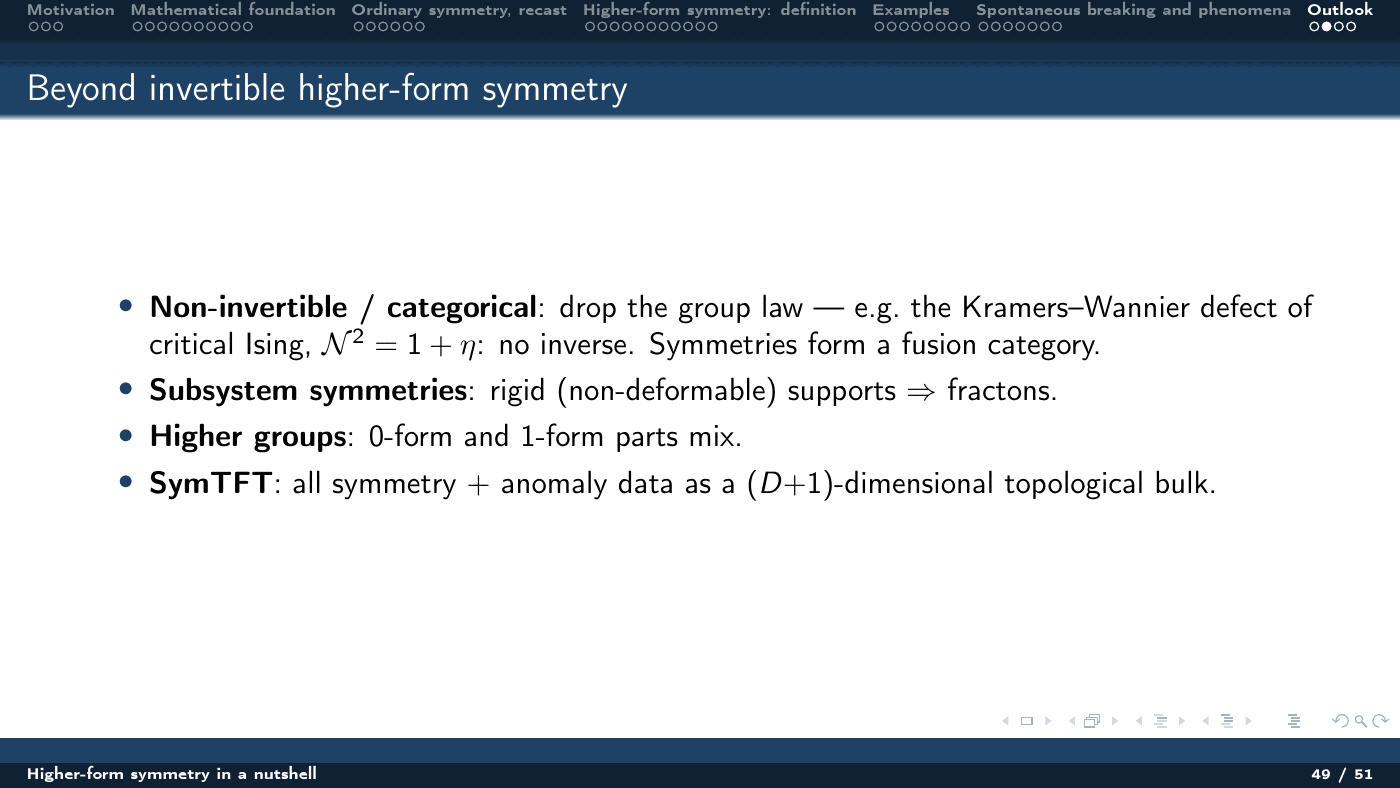
• Non-invertible / categorical. Drop the group law — the Kramers–Wannier defect of critical Ising satisfies $\mathcal{N}^2 = 1+\eta$ and has no inverse. Symmetries form a fusion category.
• Subsystem symmetries. Rigid, non-deformable supports, giving fractons.
• Higher groups. The 0-form and 1-form parts mix.
• SymTFT. All symmetry and anomaly data repackaged as a $(D{+}1)$-dimensional topological bulk.

Summary

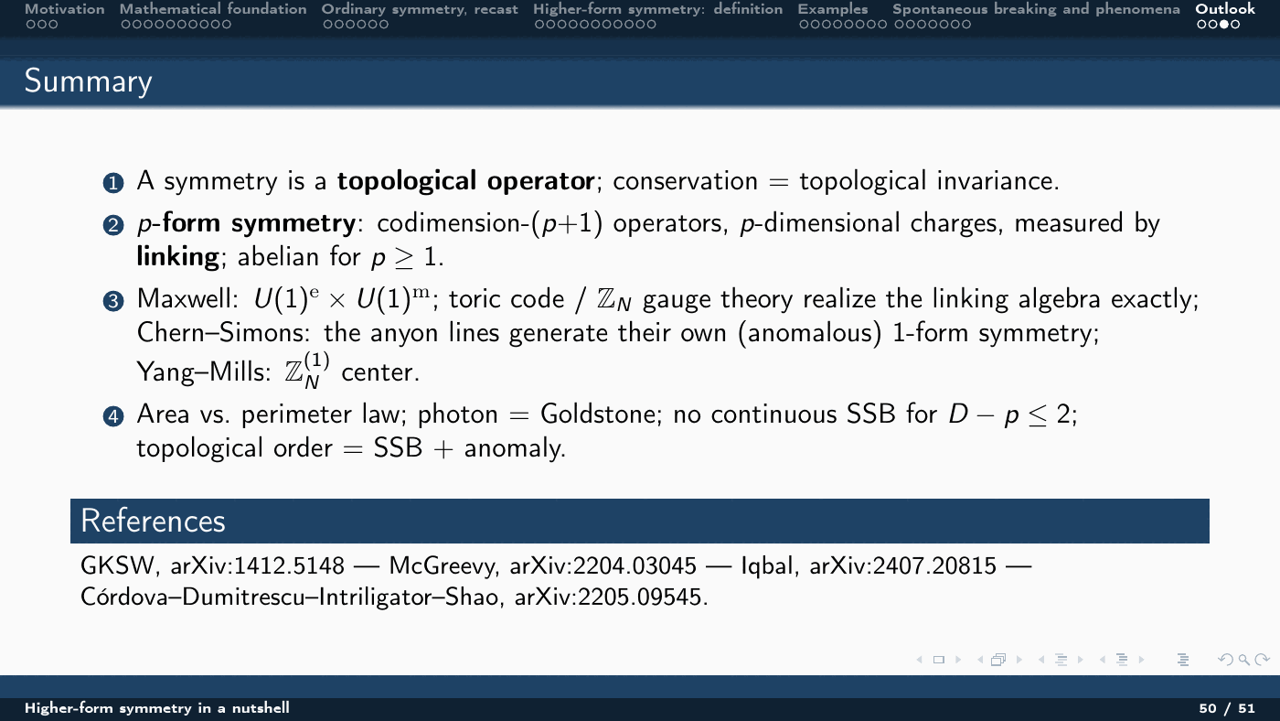
1. A symmetry is a topological operator; conservation is topological invariance.
2. A $p$-form symmetry has codimension-$(p+1)$ operators and $p$-dimensional charges, measured by linking, and is abelian for $p\ge 1$.
3. Maxwell realizes $U(1)_e\times U(1)_m$; the toric code and $\mathbb{Z}_N$ gauge theory realize the linking algebra exactly; in Chern–Simons the anyon lines generate their own (anomalous) 1-form symmetry; Yang–Mills carries the $\mathbb{Z}_N^{(1)}$ center.
4. Area versus perimeter law; the photon as a Goldstone boson; no continuous SSB for $D-p\le 2$; topological order as SSB plus anomaly.

References

1. D. Gaiotto, A. Kapustin, N. Seiberg, B. Willett, “Generalized Global Symmetries,” arXiv:1412.5148.
2. J. McGreevy, “Generalized Symmetries in Condensed Matter,” arXiv:2204.03045.
3. N. Iqbal, “Jena lectures on generalized global symmetries,” arXiv:2407.20815.
4. C. Córdova, T. T. Dumitrescu, K. Intriligator, S.-H. Shao, “Snowmass White Paper: Generalized Symmetries in Quantum Field Theory and Beyond,” arXiv:2205.09545.