Density Matrix Geometry and Response Functions

Presenter	Yuntao Guan (Prof. Barry Bradlyn’s group, UIUC)
Date	September 28, 2026 · 4:30–6:00 PM
Location	Davey 339
Topic	Density matrix geometry and response functions
Papers	Y. Guan and B. Bradlyn, Phys. Rev. Research 8, 013291 (2026); B. Bradlyn, arXiv:2608.06326 (2026)

The quantum geometric tensor packs the Berry curvature and the quantum metric into one object, and it has become a standard tool for Hall responses, Wannier localization, flat-band superconductivity and optical sum rules. But the usual version has four limitations. It is a linear-order object. It lives at zero temperature. And it is tied either to Bloch bands of noninteracting electrons or to twist angles of an interacting ground state. The talk replaces the pure state by the density matrix, and the quantum distance by the Bures distance between the thermal state and the state driven by an arbitrary time-dependent field. Expanding that distance in the field strength defines a Bures metric at second order and a Bures connection at third order, and both come out as explicit spectral functions. Specific limits of the metric recover earlier results: a finite-temperature Souza–Wilkens–Martin (SWM) sum rule, the quantum Fisher information, and Fermi’s golden rule recast as geometry. At zero temperature, the connection reduces to the band-theory Christoffel symbol. The second half follows the connection into nonlinear optics. The sum rule for the shift current contains a genuinely multi-state term, built from transitions between two excited states. That term is the non-metricity of the mixture/exponential connections of quantum information geometry.

Part 1 — Background: the quantum geometric tensor

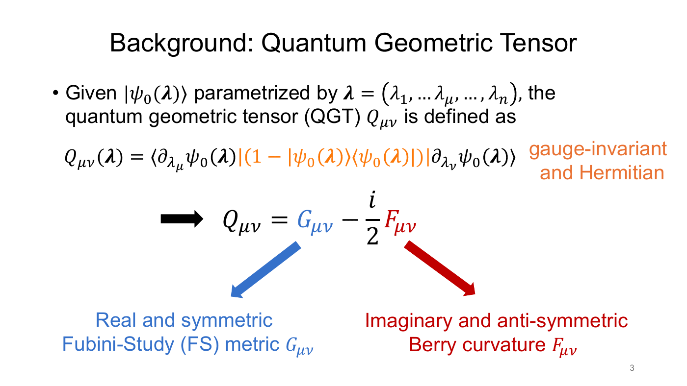
Take a normalized state $\lvert\psi_0(\boldsymbol\lambda)\rangle$ that depends on parameters $\boldsymbol\lambda = (\lambda_1,\dots,\lambda_n)$. Its quantum geometric tensor (QGT) is

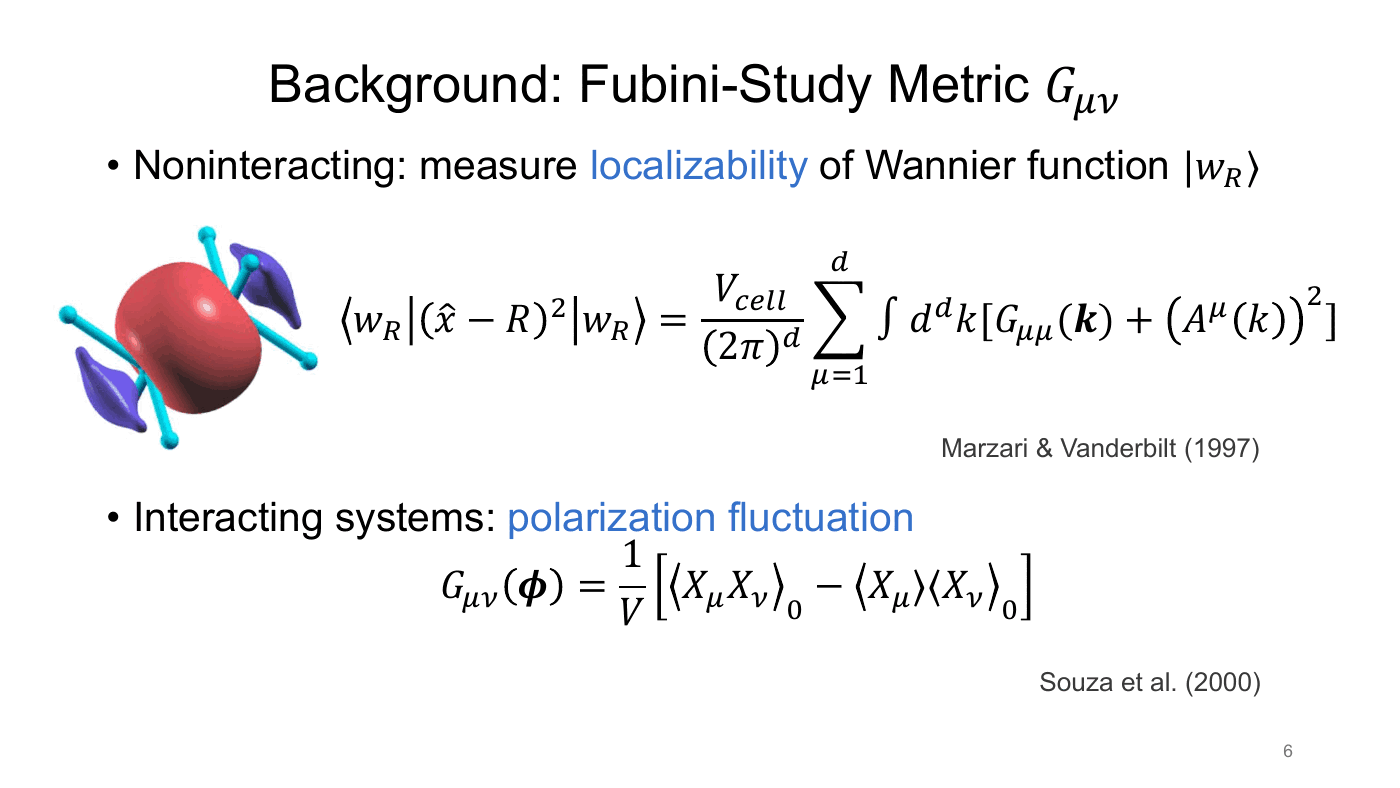
$$ Q_{\mu\nu}(\boldsymbol\lambda) = \langle\partial_{\lambda_\mu}\psi_0\rvert\big(1-\lvert\psi_0\rangle\langle\psi_0\rvert\big)\lvert\partial_{\lambda_\nu}\psi_0\rangle = G_{\mu\nu} - \frac{i}{2}F_{\mu\nu}. $$

The projector makes $Q$ gauge-invariant, and $Q$ is Hermitian. Its real, symmetric part is the Fubini–Study metric $G_{\mu\nu}$. Its imaginary, antisymmetric part is the Berry curvature $F_{\mu\nu}$.

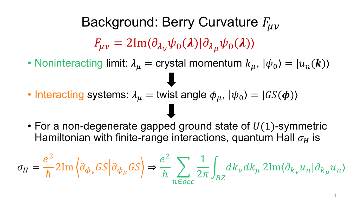
Berry curvature. $F_{\mu\nu} = 2\,\mathrm{Im}\,\langle\partial_{\lambda_\nu}\psi_0\vert\partial_{\lambda_\mu}\psi_0\rangle$. For noninteracting electrons, the parameters are the crystal momenta and the state is a Bloch function, $\lvert u_n(\mathbf k)\rangle$. For interacting systems, they are the twist angles $\phi_\mu$ of the boundary conditions, and the state is the ground state $\lvert GS(\boldsymbol\phi)\rangle$. Take a non-degenerate gapped ground state of a $U(1)$-symmetric Hamiltonian with finite-range interactions. Its Hall conductance is the twist-angle Berry curvature, which reduces to the TKNN formula in the band limit:

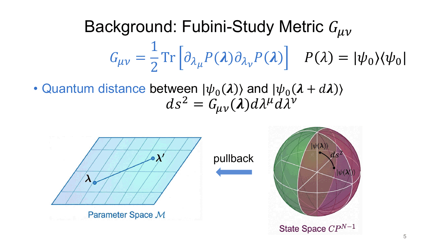
$$ \sigma_H = \frac{e^2}{\hbar}\,2\,\mathrm{Im}\,\langle\partial_{\phi_\nu}GS\vert\partial_{\phi_\mu}GS\rangle \;\Rightarrow\; \frac{e^2}{h}\sum_{n\in\text{occ}}\frac{1}{2\pi}\int_{BZ}\mathrm dk_\nu\,\mathrm dk_\mu\; 2\,\mathrm{Im}\,\langle\partial_{k_\nu}u_n\vert\partial_{k_\mu}u_n\rangle . $$

Fubini–Study metric. With the projector $P(\boldsymbol\lambda) = \lvert\psi_0\rangle\langle\psi_0\rvert$, the metric is $G_{\mu\nu} = \tfrac12\operatorname{Tr}\big[\partial_{\lambda_\mu}P\,\partial_{\lambda_\nu}P\big]$. It measures the quantum distance between neighbouring states, $\mathrm ds^2 = G_{\mu\nu}\,\mathrm d\lambda^\mu\mathrm d\lambda^\nu$. In other words, it is the pullback of the natural metric on state space $\mathbb{CP}^{N-1}$ to parameter space. It controls two physical quantities:

• Noninteracting: the spread of Wannier functions (Marzari–Vanderbilt 1997), $$ \langle w_R\rvert(\hat x - R)^2\lvert w_R\rangle = \frac{V_{\text{cell}}}{(2\pi)^d}\sum_{\mu=1}^d\int\mathrm d^dk\,\big[G_{\mu\mu}(\mathbf k) + (A^\mu(\mathbf k))^2\big]. $$
• Interacting: the fluctuation of the polarization (Souza et al. 2000), $G_{\mu\nu}(\boldsymbol\phi) = \frac1V\big[\langle X_\mu X_\nu\rangle_0 - \langle X_\mu\rangle_0\langle X_\nu\rangle_0\big]$.

Some applications.

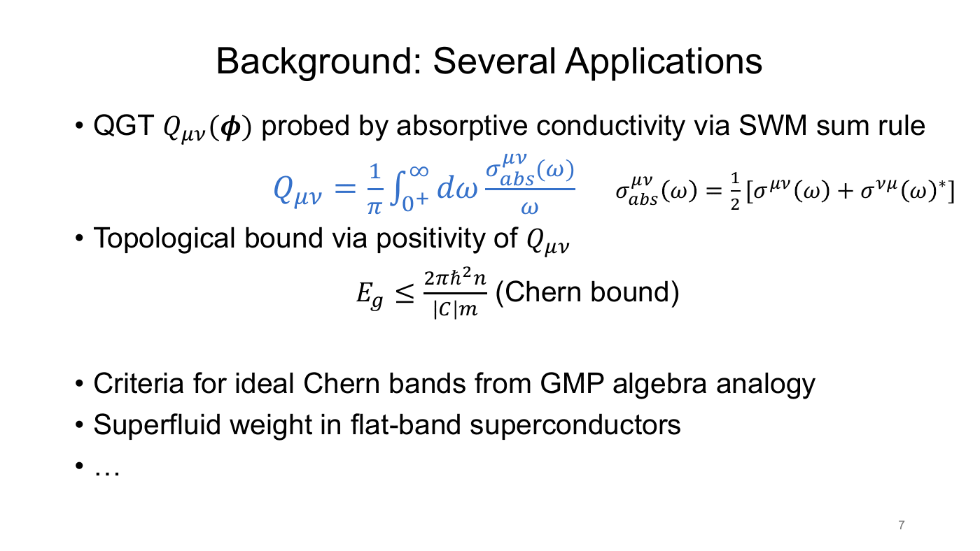
• The SWM sum rule measures the QGT through the absorptive conductivity: $$ Q_{\mu\nu} = \frac1\pi\int_{0^+}^\infty\mathrm d\omega\,\frac{\sigma^{\mu\nu}_{\text{abs}}(\omega)}{\omega}, \qquad \sigma^{\mu\nu}_{\text{abs}}(\omega) = \tfrac12\big[\sigma^{\mu\nu}(\omega) + \sigma^{\nu\mu}(\omega)^*\big]. $$
• Positivity of $Q_{\mu\nu}$ gives a topological bound on the gap, the Chern bound $E_g \le 2\pi\hbar^2 n/(\lvert C\rvert m)$.
• Also: criteria for ideal Chern bands (from an analogy with the GMP algebra), and the superfluid weight of flat-band superconductors.

Part 2 — Motivation: four limitations

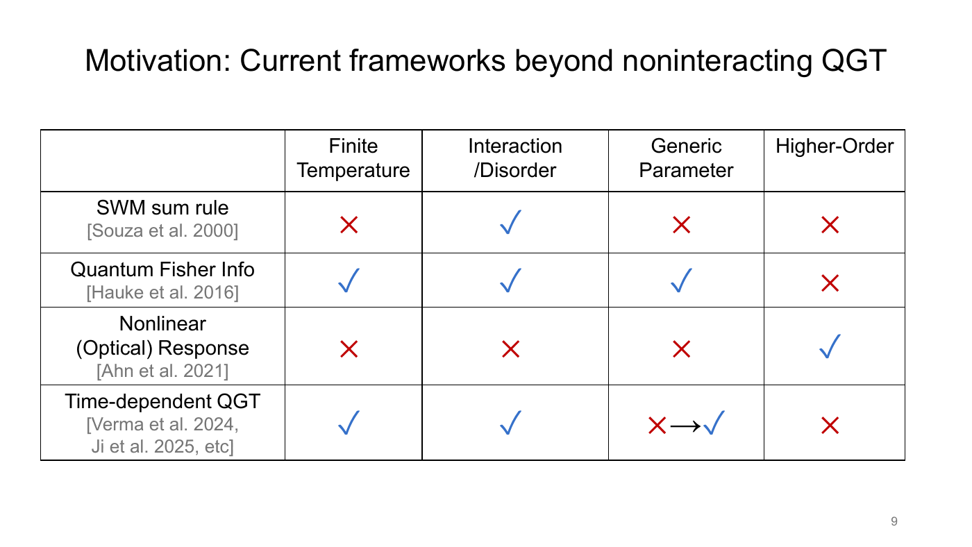
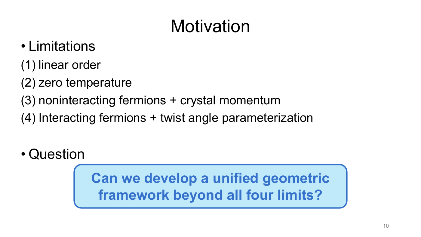
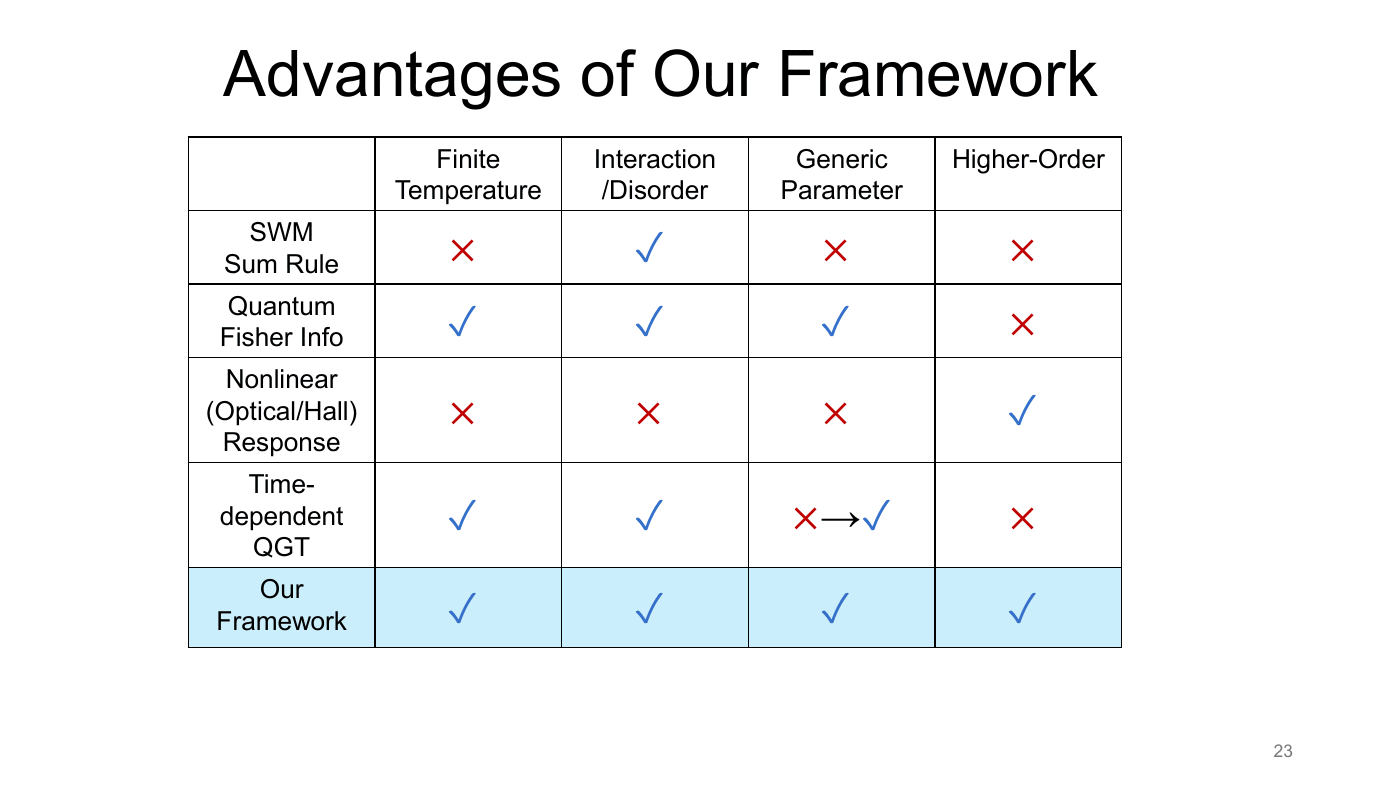
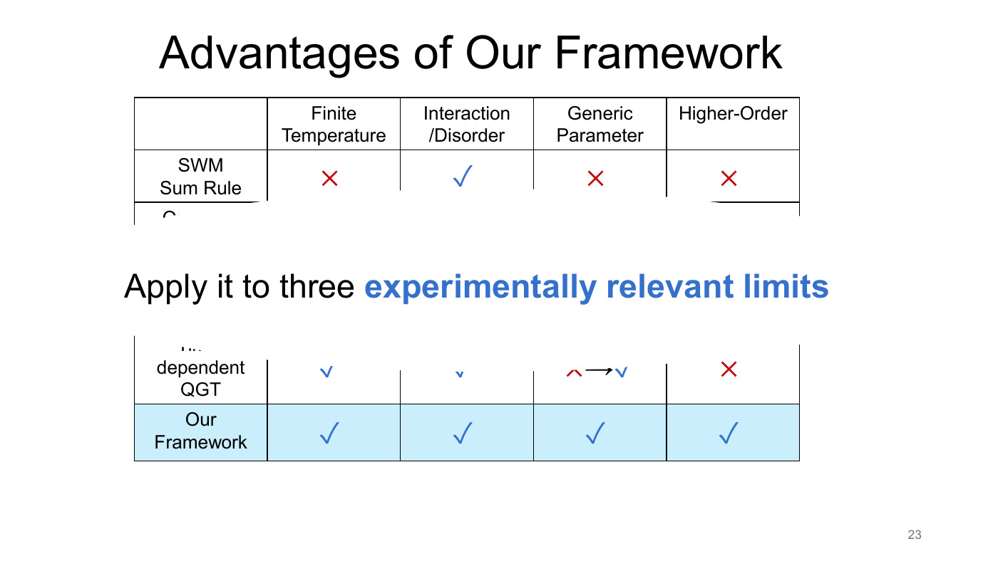
The standard QGT is restricted to (1) linear order, (2) zero temperature, and either (3) noninteracting fermions parameterized by crystal momentum or (4) interacting fermions parameterized by twist angles. Several existing frameworks each lift some of these limits, but none lifts all of them:

Framework	Finite $T$	Interaction / disorder	Generic parameter	Higher order
SWM sum rule [Souza et al. 2000]	✗	✓	✗	✗
Quantum Fisher information [Hauke et al. 2016]	✓	✓	✓	✗
Nonlinear (optical) response [Ahn et al. 2021]	✗	✗	✗	✓
Time-dependent QGT [Verma et al. 2024; Ji et al. 2025]	✓	✓	✗ → ✓	✗

The question of the talk: can one build a single geometric framework that goes beyond all four limits?

Part 3 — Bures distance

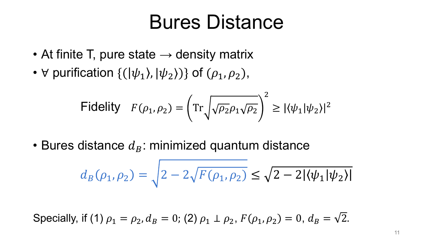
At finite temperature, the pure state becomes a density matrix. The fidelity of two density matrices is the best overlap achievable by any pair of purifications $(\lvert\psi_1\rangle,\lvert\psi_2\rangle)$ of $(\rho_1,\rho_2)$:

$$ F(\rho_1,\rho_2) = \Big(\operatorname{Tr}\sqrt{\sqrt{\rho_2}\,\rho_1\sqrt{\rho_2}}\Big)^2 \;\ge\; \lvert\langle\psi_1\vert\psi_2\rangle\rvert^2 . $$

The Bures distance is the corresponding minimized quantum distance:

$$ d_B(\rho_1,\rho_2) = \sqrt{2-2\sqrt{F(\rho_1,\rho_2)}} \;\le\; \sqrt{2-2\lvert\langle\psi_1\vert\psi_2\rangle\rvert}. $$

It vanishes for $\rho_1 = \rho_2$ and reaches its maximum $\sqrt2$ for orthogonal states, where $F = 0$.

Part 4 — Expanding the Bures distance

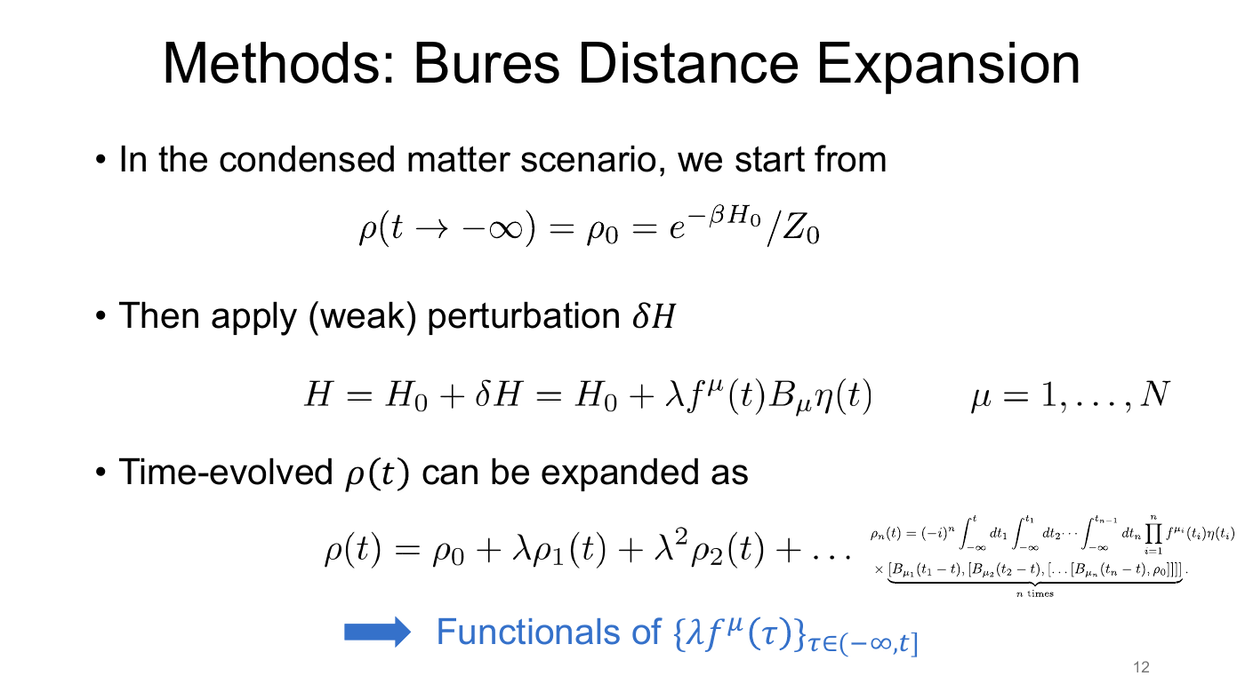
Setup. Start in thermal equilibrium, $\rho(t\to-\infty) = \rho_0 = e^{-\beta H_0}/Z_0$. Then switch on a weak perturbation along $N$ operator directions $B_\mu$,

$$ H = H_0 + \lambda f^\mu(t)\,B_\mu\,\eta(t),\qquad \mu = 1,\dots,N, $$

where $\eta(t)$ switches the perturbation on adiabatically. The time-evolved density matrix has a Dyson expansion, $\rho(t) = \rho_0 + \lambda\rho_1(t) + \lambda^2\rho_2(t) + \dots$, with nested commutators

$$ \begin{aligned} \rho_n(t) = (-i)^n&\int_{-\infty}^t\!\mathrm dt_1\cdots\int_{-\infty}^{t_{n-1}}\!\mathrm dt_n \prod_{i=1}^n f^{\mu_i}(t_i)\,\eta(t_i) \\ &\times\big[B_{\mu_1}(t_1-t),\big[B_{\mu_2}(t_2-t),\big[\dots\big[B_{\mu_n}(t_n-t),\rho_0\big]\big]\big]\big]. \end{aligned} $$

So $\rho(t)$ is a functional of the whole field history $\{\lambda f^\mu(\tau)\}_{\tau\in(-\infty,t]}$. The central object is

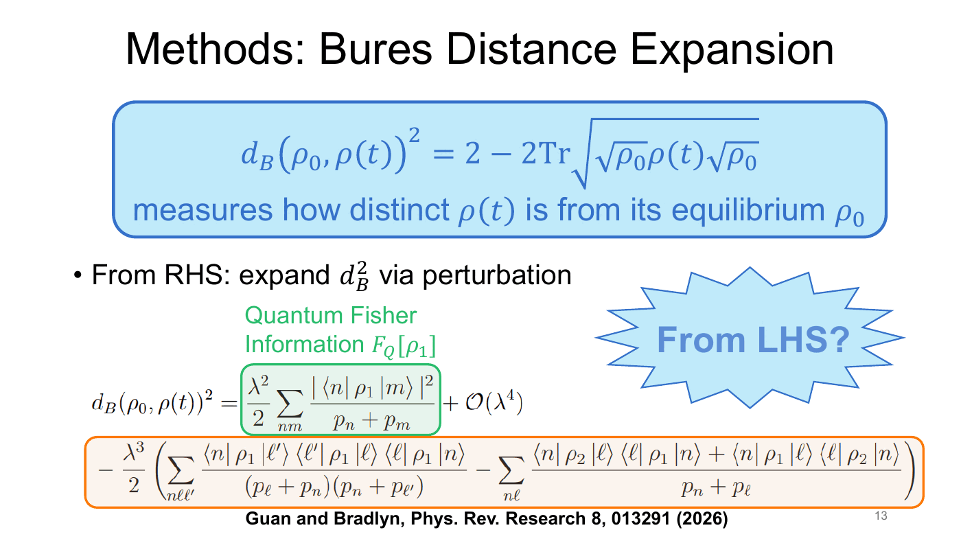
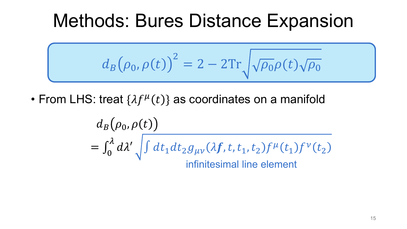
$$ d_B\big(\rho_0,\rho(t)\big)^2 = 2 - 2\operatorname{Tr}\sqrt{\sqrt{\rho_0}\,\rho(t)\sqrt{\rho_0}} , $$

which measures how far the driven state has moved from equilibrium. The idea is to compute it in two different ways and compare.

From the right-hand side (perturbation theory). In the eigenbasis of $\rho_0 = \sum_n p_n\lvert n\rangle\langle n\rvert$,

$$ \begin{aligned} d_B(\rho_0,\rho(t))^2 &= \frac{\lambda^2}{2}\sum_{nm}\frac{\lvert\langle n\rvert\rho_1\lvert m\rangle\rvert^2}{p_n+p_m} \\ &\quad - \frac{\lambda^3}{2}\Bigg(\sum_{n\ell\ell'}\frac{\langle n\rvert\rho_1\lvert\ell'\rangle\langle\ell'\rvert\rho_1\lvert\ell\rangle\langle\ell\rvert\rho_1\lvert n\rangle}{(p_\ell+p_n)(p_n+p_{\ell'})} - {} \\ &\qquad\quad \sum_{n\ell}\frac{\langle n\rvert\rho_2\lvert\ell\rangle\langle\ell\rvert\rho_1\lvert n\rangle + \langle n\rvert\rho_1\lvert\ell\rangle\langle\ell\rvert\rho_2\lvert n\rangle}{p_n+p_\ell}\Bigg) + \mathcal O(\lambda^4). \end{aligned} $$

The $\lambda^2$ term is the quantum Fisher information $F_Q[\rho_1]$ (up to normalization).

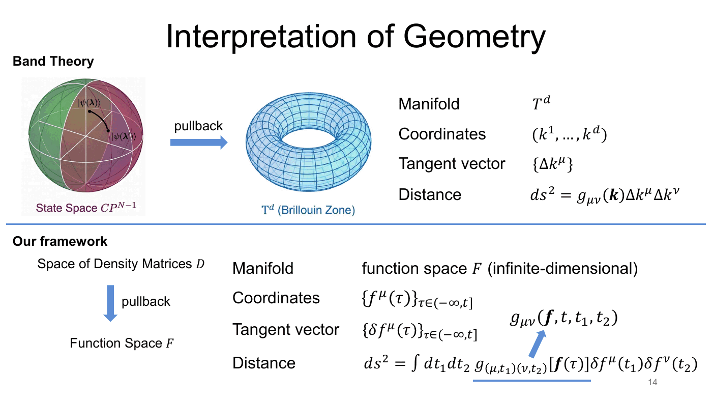
From the left-hand side (geometry). Treat the field history itself as coordinates. The manifold is now an infinite-dimensional function space, with coordinates $\{f^\mu(\tau)\}_{\tau\in(-\infty,t]}$ and tangent vectors $\{\delta f^\mu(\tau)\}$. The density matrices are pulled back to it, just as band theory pulls $\mathbb{CP}^{N-1}$ back to the Brillouin-zone torus $T^d$. The line element becomes a double time integral,

$$ \mathrm ds^2 = \int\mathrm dt_1\,\mathrm dt_2\; g_{(\mu,t_1)(\nu,t_2)}[\boldsymbol f(\tau)]\;\delta f^\mu(t_1)\,\delta f^\nu(t_2), $$

and the Bures distance is the length of the straight path from $0$ to $\lambda\boldsymbol f$:

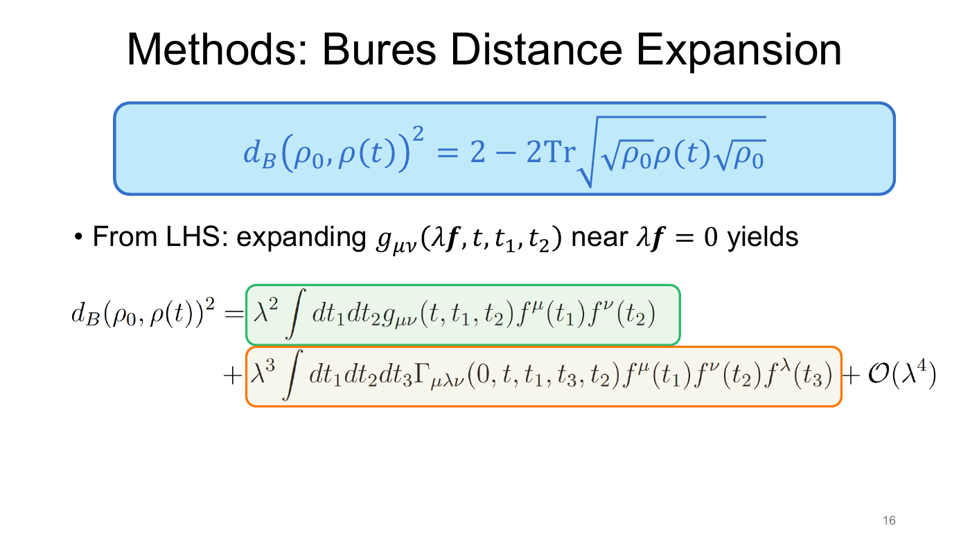
$$ d_B\big(\rho_0,\rho(t)\big) = \int_0^\lambda\mathrm d\lambda'\, \sqrt{\int\mathrm dt_1\,\mathrm dt_2\;g_{\mu\nu}(\lambda'\boldsymbol f,t,t_1,t_2)\,f^\mu(t_1)f^\nu(t_2)} . $$

Expanding the metric around $\lambda\boldsymbol f = 0$ gives

$$ \begin{aligned} d_B(\rho_0,\rho(t))^2 &= \lambda^2\int\mathrm dt_1\mathrm dt_2\;g_{\mu\nu}(t,t_1,t_2)\,f^\mu(t_1)f^\nu(t_2) \\ &\quad + \lambda^3\int\mathrm dt_1\mathrm dt_2\mathrm dt_3\;\Gamma_{\mu\lambda\nu}(0,t,t_1,t_3,t_2)\,f^\mu(t_1)f^\nu(t_2)f^\lambda(t_3) \\ &\quad + \mathcal O(\lambda^4). \end{aligned} $$

The $\lambda^2$ coefficient is a metric, and the $\lambda^3$ coefficient is a connection.

Order $\lambda^2$: the Bures metric

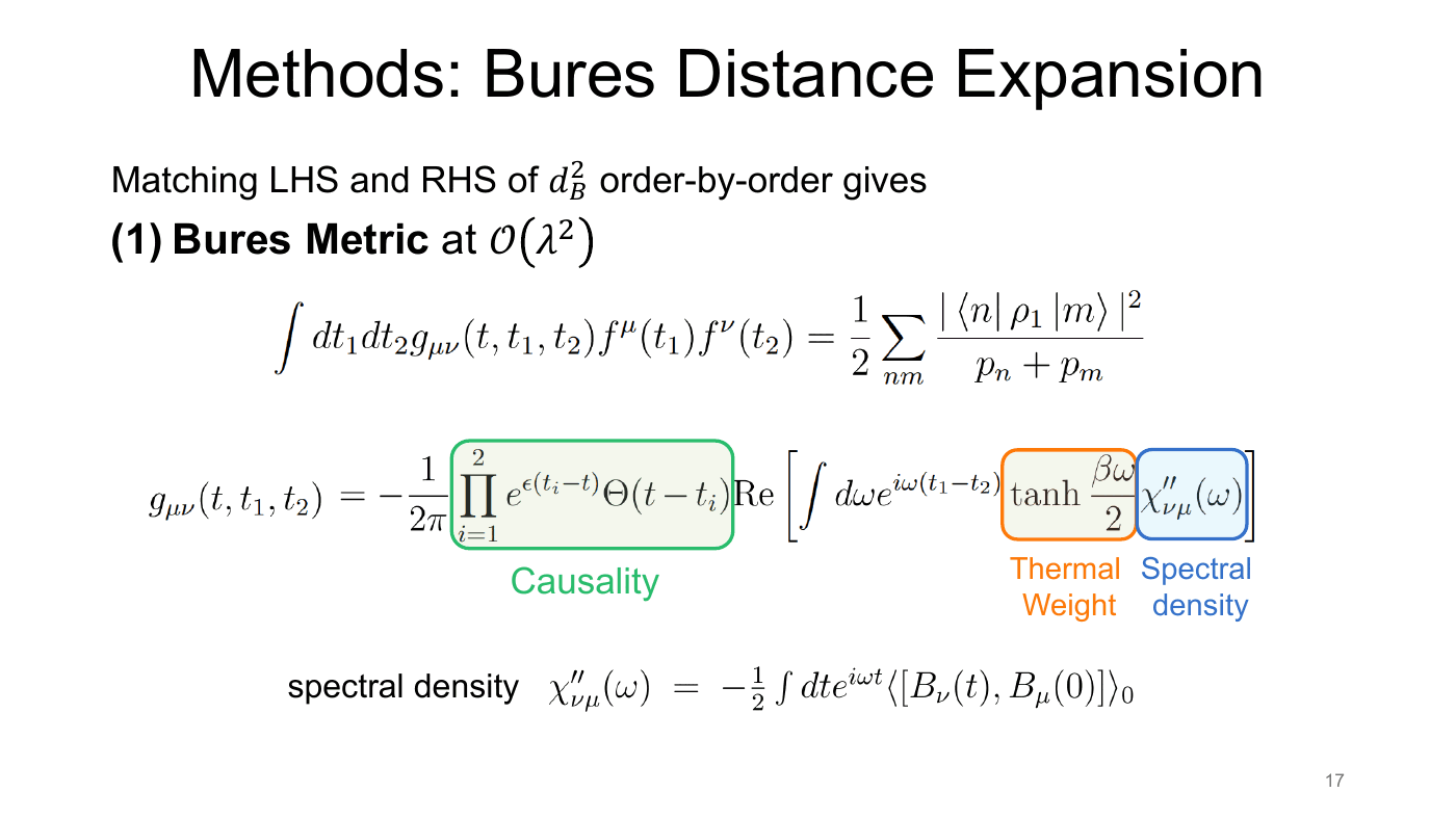
Matching the two expansions at second order identifies the metric with the Fisher term:

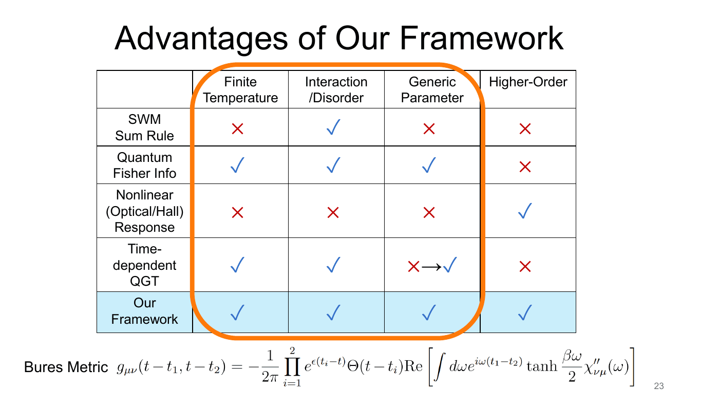
$$ g_{\mu\nu}(t,t_1,t_2) = -\frac{1}{2\pi}\prod_{i=1}^2 e^{\epsilon(t_i-t)}\,\Theta(t-t_i)\; \mathrm{Re}\Big[\int\mathrm d\omega\,e^{i\omega(t_1-t_2)}\tanh\frac{\beta\omega}{2}\,\chi''_{\nu\mu}(\omega)\Big], $$$$ \chi''_{\nu\mu}(\omega) = -\frac12\int\mathrm dt\,e^{i\omega t}\,\big\langle[B_\nu(t),B_\mu(0)]\big\rangle_0 . $$

Each factor has a clear job. The step functions encode causality: only field values before $t$ matter. The factor $\tanh(\beta\omega/2)$ is the thermal weight. The spectral density $\chi''$ carries the dynamics of the system. Everything is expressed through a measurable response function, with no assumption about bands or ground states.

Order $\lambda^3$: the Bures connection

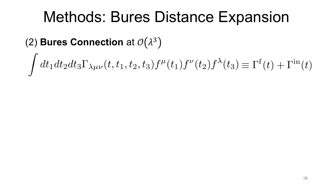
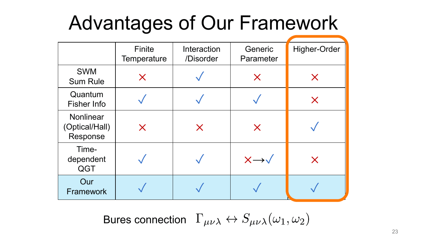
At third order the coefficient splits into two pieces, $\int\Gamma_{\lambda\mu\nu}\,f^\mu f^\nu f^\lambda \equiv \Gamma^{\text f}(t) + \Gamma^{\text{in}}(t)$.

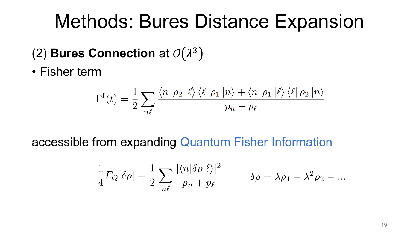
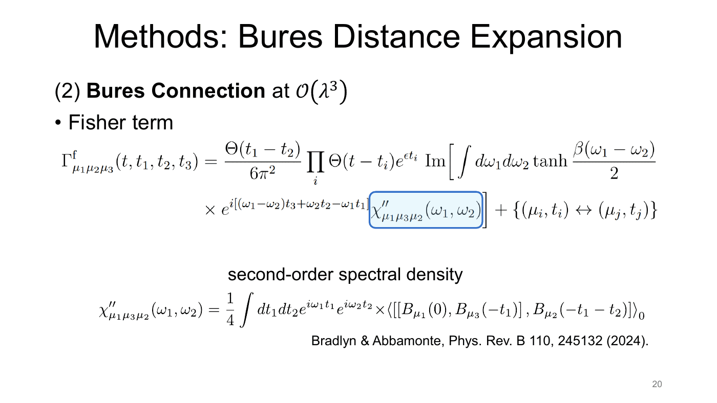
• Fisher term. This piece comes from expanding the quantum Fisher information of $\delta\rho = \lambda\rho_1 + \lambda^2\rho_2 + \dots$ to the next order: $$ \Gamma^{\text f}(t) = \frac12\sum_{n\ell}\frac{\langle n\rvert\rho_2\lvert\ell\rangle\langle\ell\rvert\rho_1\lvert n\rangle + \langle n\rvert\rho_1\lvert\ell\rangle\langle\ell\rvert\rho_2\lvert n\rangle}{p_n+p_\ell}. $$ In the time domain, it is a tanh-weighted transform of the second-order spectral density (Bradlyn & Abbamonte 2024), $$ \begin{aligned} \chi''_{\mu_1\mu_3\mu_2}(\omega_1,\omega_2) &= \frac14\int\mathrm dt_1\mathrm dt_2\,e^{i\omega_1t_1}e^{i\omega_2t_2} \\ &\quad\times\big\langle\big[[B_{\mu_1}(0),B_{\mu_3}(-t_1)],B_{\mu_2}(-t_1-t_2)\big]\big\rangle_0 , \end{aligned} $$ with weight $\tanh\frac{\beta(\omega_1-\omega_2)}{2}$.
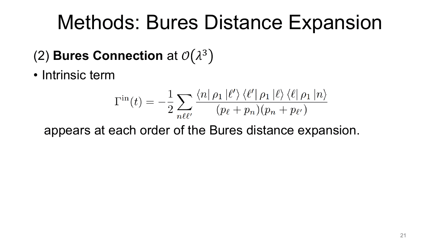
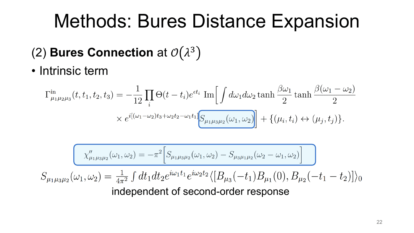
• Intrinsic term. This piece has no Fisher-information counterpart, and it appears at every order of the expansion: $$ \Gamma^{\text{in}}(t) = -\frac12\sum_{n\ell\ell'}\frac{\langle n\rvert\rho_1\lvert\ell'\rangle\langle\ell'\rvert\rho_1\lvert\ell\rangle\langle\ell\rvert\rho_1\lvert n\rangle}{(p_\ell+p_n)(p_n+p_{\ell'})}. $$ In the time domain it carries a double weight $\tanh\frac{\beta\omega_1}{2}\tanh\frac{\beta(\omega_1-\omega_2)}{2}$, applied to a new three-point function, $$ \begin{aligned} S_{\mu_1\mu_3\mu_2}(\omega_1,\omega_2) &= \frac{1}{4\pi^2}\int\mathrm dt_1\mathrm dt_2\,e^{i\omega_1t_1}e^{i\omega_2t_2} \\ &\quad\times\big\langle\big[B_{\mu_3}(-t_1)B_{\mu_1}(0),\,B_{\mu_2}(-t_1-t_2)\big]\big\rangle_0 . \end{aligned} $$ Only an antisymmetrized combination of $S$ is fixed by the second-order response, $\chi''_{\mu_1\mu_3\mu_2}(\omega_1,\omega_2) = -\pi^2\big[S_{\mu_1\mu_3\mu_2}(\omega_1,\omega_2) - S_{\mu_3\mu_1\mu_2}(\omega_2-\omega_1,\omega_2)\big]$. The intrinsic term is therefore independent of the second-order response. It is new information, and Part 7 returns to it.

With both pieces in hand, the framework fills in the whole table: finite temperature, interactions and disorder, generic perturbing operators (through the metric), and higher order (through the connection).

Part 5 — Three limits of the Bures metric

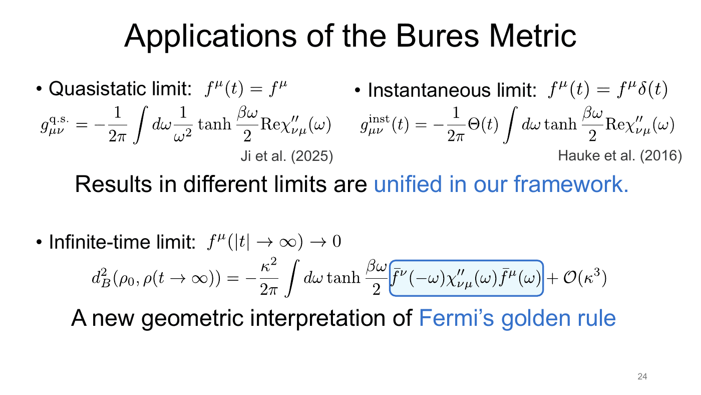
The same metric reduces to known quantities for three experimentally relevant field profiles.

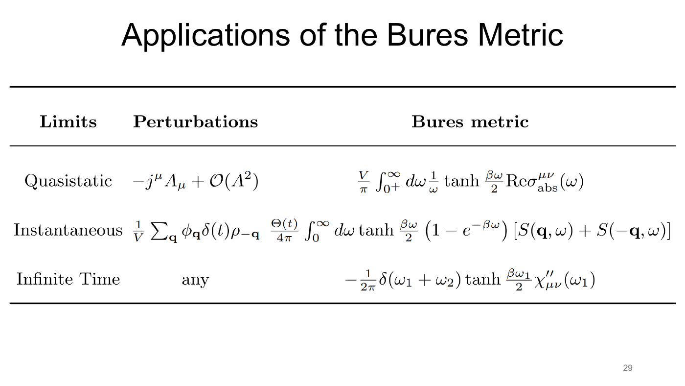
Limit	Field profile	Example perturbation	The metric becomes
Quasistatic	$f^\mu(t)\to f^\mu$	current, $-j^\mu A_\mu + \mathcal O(A^2)$	finite-$T$ SWM sum rule
Instantaneous	$f^\mu(t) = f^\mu\delta(t)$	density kick	quantum Fisher information
Infinite time	$f^\mu(\pm\infty)\to0$, $t\to+\infty$	any pulse	Fermi’s golden rule

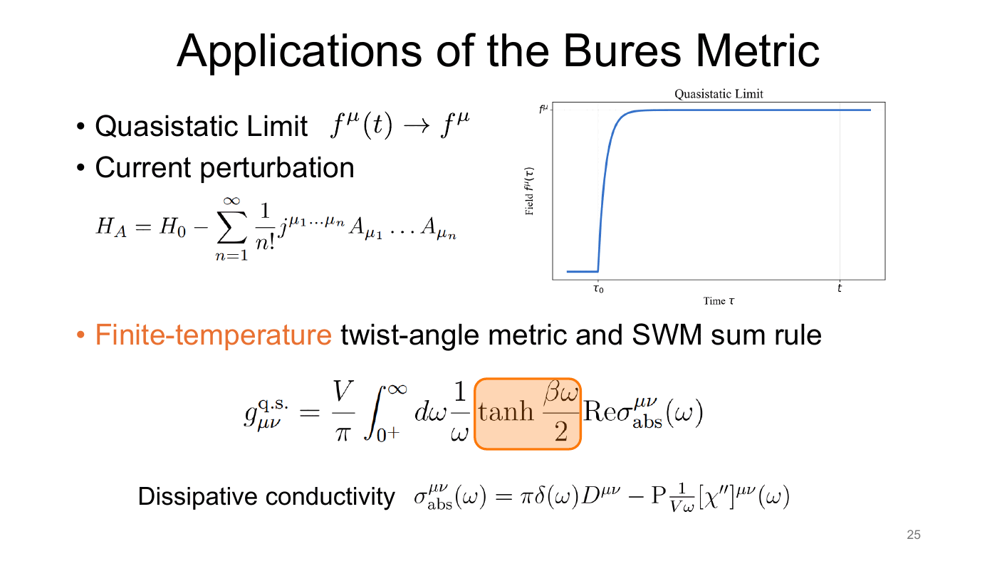
Quasistatic limit. The field ramps up and then stays constant. In general,

$$ g^{\text{q.s.}}_{\mu\nu} = -\frac1{2\pi}\int\mathrm d\omega\,\frac1{\omega^2}\tanh\frac{\beta\omega}{2}\,\mathrm{Re}\,\chi''_{\nu\mu}(\omega), $$

which is the result of Ji et al. (2025). Now take a current perturbation, $H_A = H_0 - \sum_n\frac1{n!}j^{\mu_1\cdots\mu_n}A_{\mu_1}\cdots A_{\mu_n}$. The metric becomes a finite-temperature twist-angle metric, which is a thermal SWM sum rule:

$$ g^{\text{q.s.}}_{\mu\nu} = \frac V\pi\int_{0^+}^\infty\mathrm d\omega\,\frac1\omega\tanh\frac{\beta\omega}{2}\,\mathrm{Re}\,\sigma^{\mu\nu}_{\text{abs}}(\omega). $$

The $1/\omega$ weight of the zero-temperature rule is dressed by $\tanh(\beta\omega/2)$. The dissipative conductivity is $\sigma^{\mu\nu}_{\text{abs}}(\omega) = \pi\delta(\omega)D^{\mu\nu} - \mathrm P\,\frac{1}{V\omega}[\chi'']^{\mu\nu}(\omega)$, where $D^{\mu\nu}$ is the Drude weight.

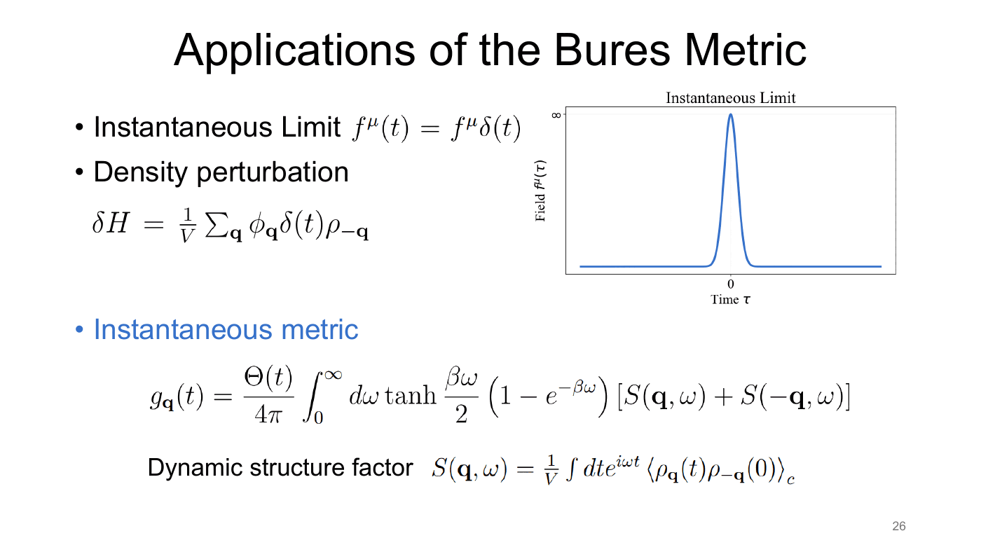
Instantaneous limit. The field is a delta-function kick. In general,

$$ g^{\text{inst}}_{\mu\nu}(t) = -\frac1{2\pi}\Theta(t)\int\mathrm d\omega\,\tanh\frac{\beta\omega}{2}\,\mathrm{Re}\,\chi''_{\nu\mu}(\omega), $$

which is the quantum Fisher information of Hauke et al. (2016). For a density kick, $\delta H = \frac1V\sum_{\mathbf q}\phi_{\mathbf q}\delta(t)\rho_{-\mathbf q}$, it is a thermally weighted integral of the dynamic structure factor $S(\mathbf q,\omega) = \frac1V\int\mathrm dt\,e^{i\omega t}\langle\rho_{\mathbf q}(t)\rho_{-\mathbf q}(0)\rangle_c$:

$$ g_{\mathbf q}(t) = \frac{\Theta(t)}{4\pi}\int_0^\infty\mathrm d\omega\,\tanh\frac{\beta\omega}{2}\,\big(1-e^{-\beta\omega}\big)\big[S(\mathbf q,\omega)+S(-\mathbf q,\omega)\big]. $$

The two limits are related to each other:

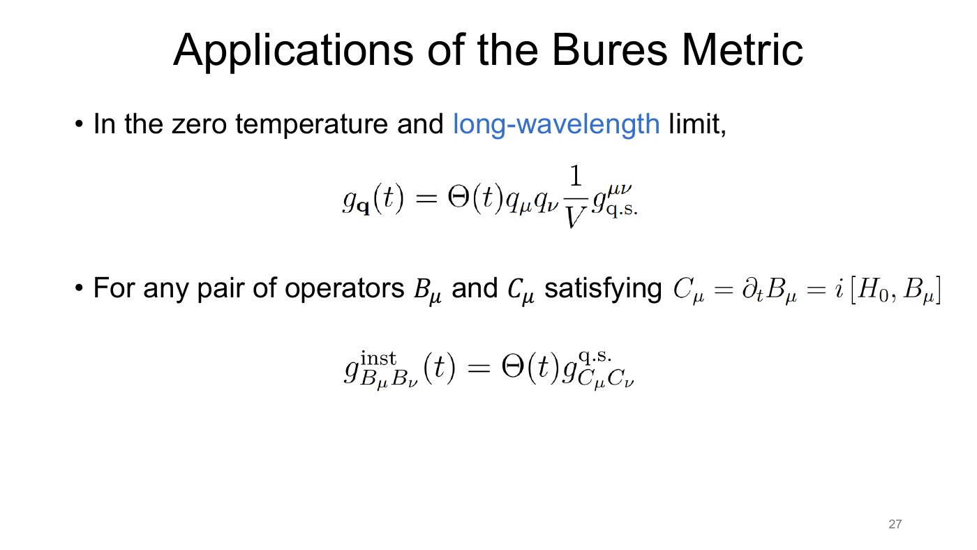
• At zero temperature and long wavelength, $g_{\mathbf q}(t) = \Theta(t)\,q_\mu q_\nu\,\frac1V\,g^{\mu\nu}_{\text{q.s.}}$.
• More generally, take any pair of operators with $C_\mu = \partial_tB_\mu = i[H_0,B_\mu]$. Then $g^{\text{inst}}_{B_\mu B_\nu}(t) = \Theta(t)\,g^{\text{q.s.}}_{C_\mu C_\nu}$: a kick in $B$ is geometrically equivalent to a quasistatic ramp in its time derivative.

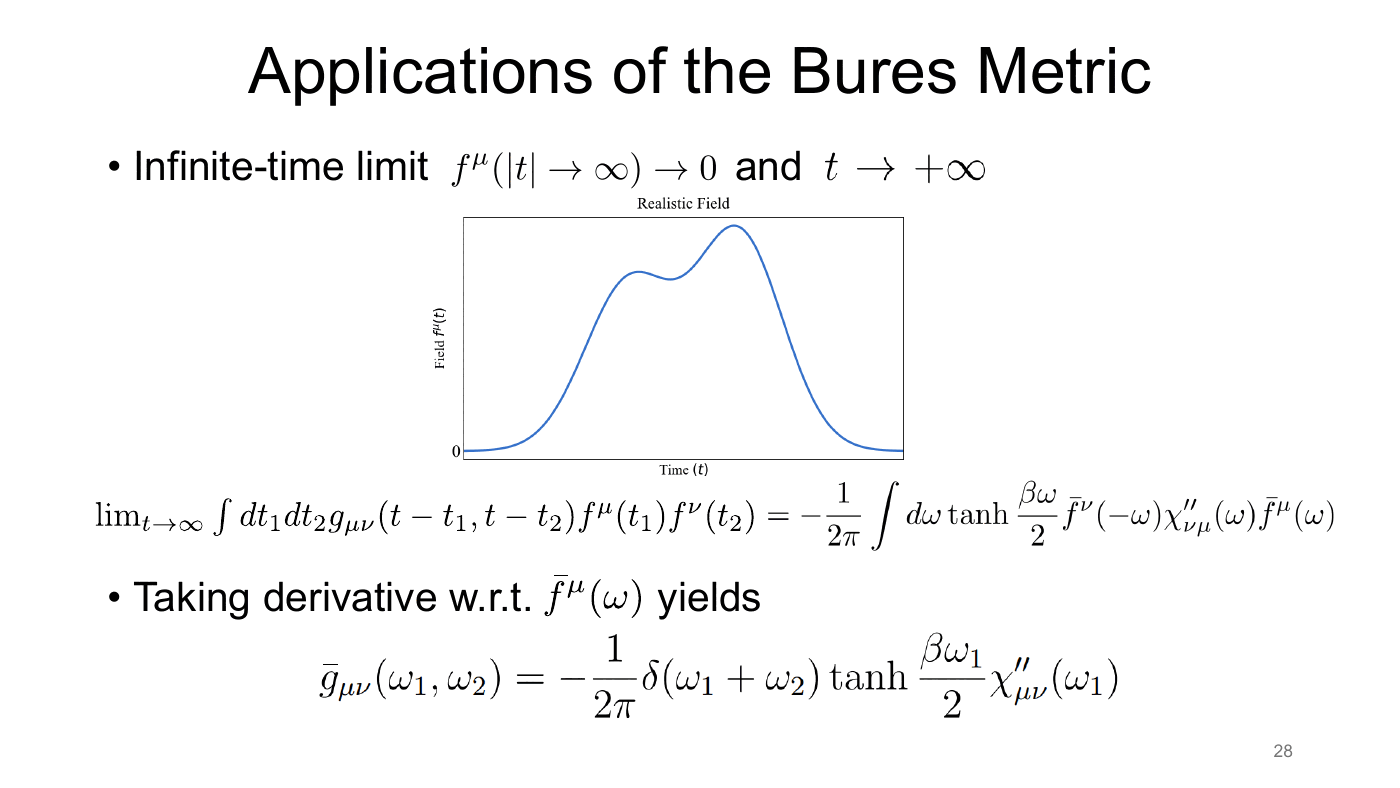
Infinite-time limit. Take a realistic pulse that vanishes in the far past and the far future, and look long after it has passed. The distance becomes

$$ \begin{aligned} d_B^2\big(\rho_0,\rho(t\to\infty)\big) &= \lim_{t\to\infty}\int\mathrm dt_1\mathrm dt_2\;g_{\mu\nu}(t-t_1,t-t_2)\,f^\mu(t_1)f^\nu(t_2) \\ &= -\frac{\kappa^2}{2\pi}\int\mathrm d\omega\,\tanh\frac{\beta\omega}{2}\;\bar f^\nu(-\omega)\,\chi''_{\nu\mu}(\omega)\,\bar f^\mu(\omega) + \mathcal O(\kappa^3), \end{aligned} $$

where $\kappa$ is the field amplitude. The integrand is exactly the absorption rate of Fermi’s golden rule, so this gives a geometric interpretation of Fermi’s golden rule: how far the pulse pushes the system away from equilibrium. Differentiating with respect to $\bar f^\mu(\omega)$ gives the frequency-space metric $\bar g_{\mu\nu}(\omega_1,\omega_2) = -\frac1{2\pi}\delta(\omega_1+\omega_2)\tanh\frac{\beta\omega_1}{2}\,\chi''_{\mu\nu}(\omega_1)$.

The three limits, previously separate results in the literature, are all special cases of one metric.

Part 6 — The Bures connection as a many-body Christoffel symbol

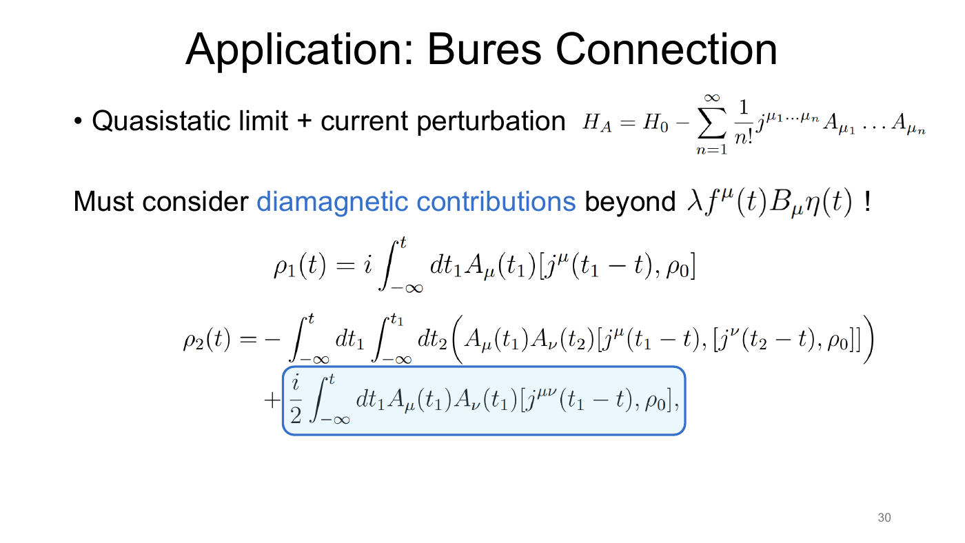
For the connection, take the quasistatic limit with a current perturbation. One subtlety matters here: the diamagnetic term $j^{\mu\nu}A_\mu A_\nu$ lies outside the linear coupling $\lambda f^\mu B_\mu$ assumed above, and it must be kept. It adds a term to $\rho_2$:

$$ \begin{aligned} \rho_2(t) &= -\int_{-\infty}^t\mathrm dt_1\int_{-\infty}^{t_1}\mathrm dt_2\;A_\mu(t_1)A_\nu(t_2)\,\big[j^\mu(t_1-t),[j^\nu(t_2-t),\rho_0]\big] \\ &\quad + \frac i2\int_{-\infty}^t\mathrm dt_1\;A_\mu(t_1)A_\nu(t_1)\,[j^{\mu\nu}(t_1-t),\rho_0], \end{aligned} $$

with $\rho_1(t) = i\int_{-\infty}^t\mathrm dt_1\,A_\mu(t_1)[j^\mu(t_1-t),\rho_0]$.

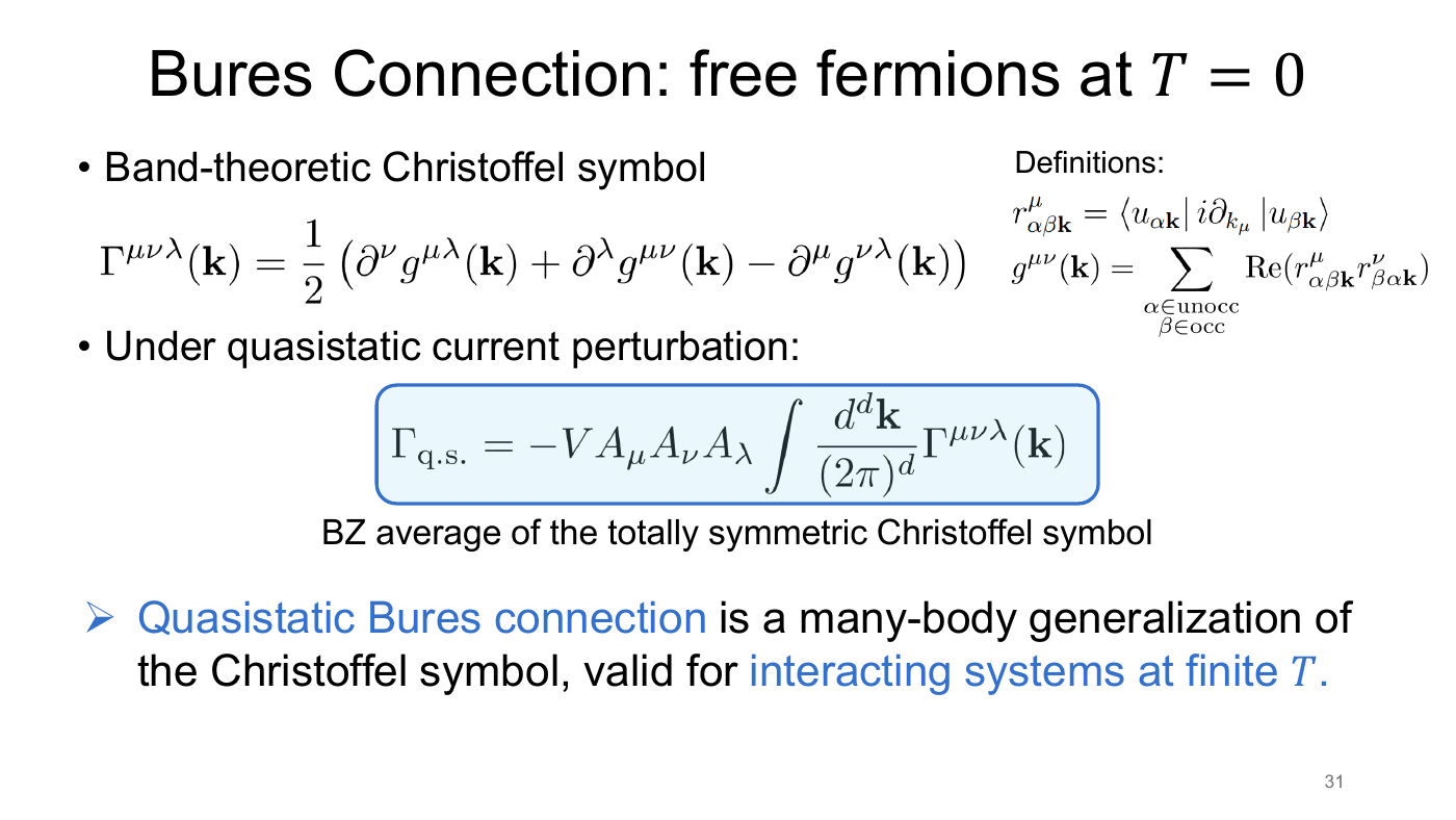
Free fermions at $T=0$. Define the band-theoretic interband Berry connection $r^\mu_{\alpha\beta\mathbf k} = \langle u_{\alpha\mathbf k}\rvert i\partial_{k_\mu}\lvert u_{\beta\mathbf k}\rangle$, the band quantum metric $g^{\mu\nu}(\mathbf k) = \sum_{\alpha\in\text{unocc},\,\beta\in\text{occ}}\mathrm{Re}\big(r^\mu_{\alpha\beta\mathbf k}r^\nu_{\beta\alpha\mathbf k}\big)$, and its Christoffel symbol

$$ \Gamma^{\mu\nu\lambda}(\mathbf k) = \frac12\big(\partial^\nu g^{\mu\lambda}(\mathbf k) + \partial^\lambda g^{\mu\nu}(\mathbf k) - \partial^\mu g^{\nu\lambda}(\mathbf k)\big). $$

The quasistatic Bures connection then reduces to the Brillouin-zone average of the Christoffel symbol, totally symmetrized by the three factors of $A$:

$$ \Gamma_{\text{q.s.}} = -V A_\mu A_\nu A_\lambda\int\frac{\mathrm d^d\mathbf k}{(2\pi)^d}\,\Gamma^{\mu\nu\lambda}(\mathbf k). $$

The quasistatic Bures connection is therefore a many-body generalization of the Christoffel symbol, and it remains valid for interacting systems at finite temperature.

Part 7 — Multi-state geometry and rectification sum rules

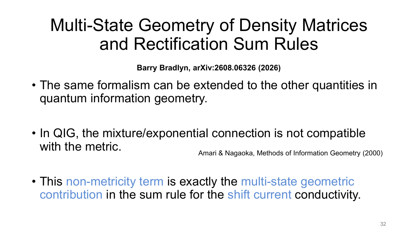
The second paper (Bradlyn, arXiv:2608.06326) extends the formalism to the rest of quantum information geometry. In information geometry, the natural mixture and exponential connections are not compatible with the metric (Amari & Nagaoka 2000). The claim is that this non-metricity is exactly the multi-state geometric contribution to the sum rule for the shift-current conductivity.

Nonlinear optics and the shift current

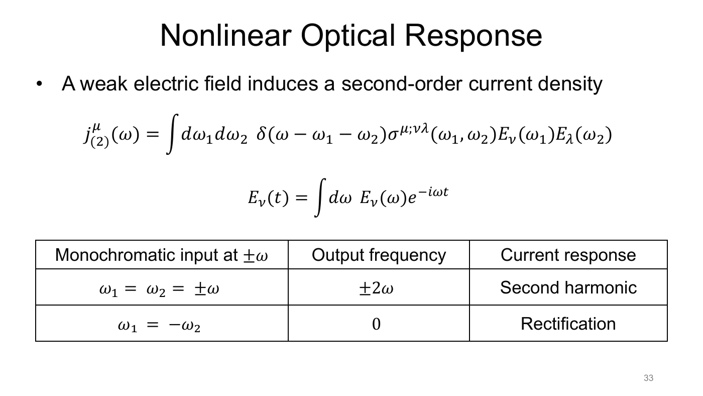
A weak electric field $E_\nu(t) = \int\mathrm d\omega\,E_\nu(\omega)e^{-i\omega t}$ induces a second-order current

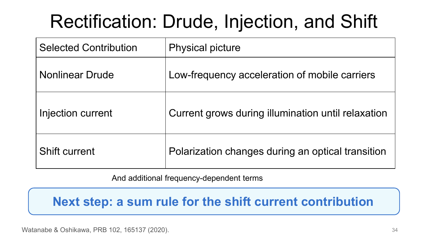
$$ j^\mu_{(2)}(\omega) = \int\mathrm d\omega_1\mathrm d\omega_2\;\delta(\omega-\omega_1-\omega_2)\,\sigma^{\mu;\nu\lambda}(\omega_1,\omega_2)\,E_\nu(\omega_1)E_\lambda(\omega_2). $$

For monochromatic light at $\pm\omega$, two channels appear. With $\omega_1 = \omega_2 = \pm\omega$ the output is at $\pm2\omega$, which is second-harmonic generation. With $\omega_1 = -\omega_2$ the output is a DC current, which is rectification. Rectification has several parts (Watanabe & Oshikawa 2020):

• the nonlinear Drude term, from low-frequency acceleration of mobile carriers;
• the injection current, which grows during illumination until relaxation cuts it off;
• the shift current, which comes from the change in polarization during an optical transition;
• plus additional frequency-dependent terms.

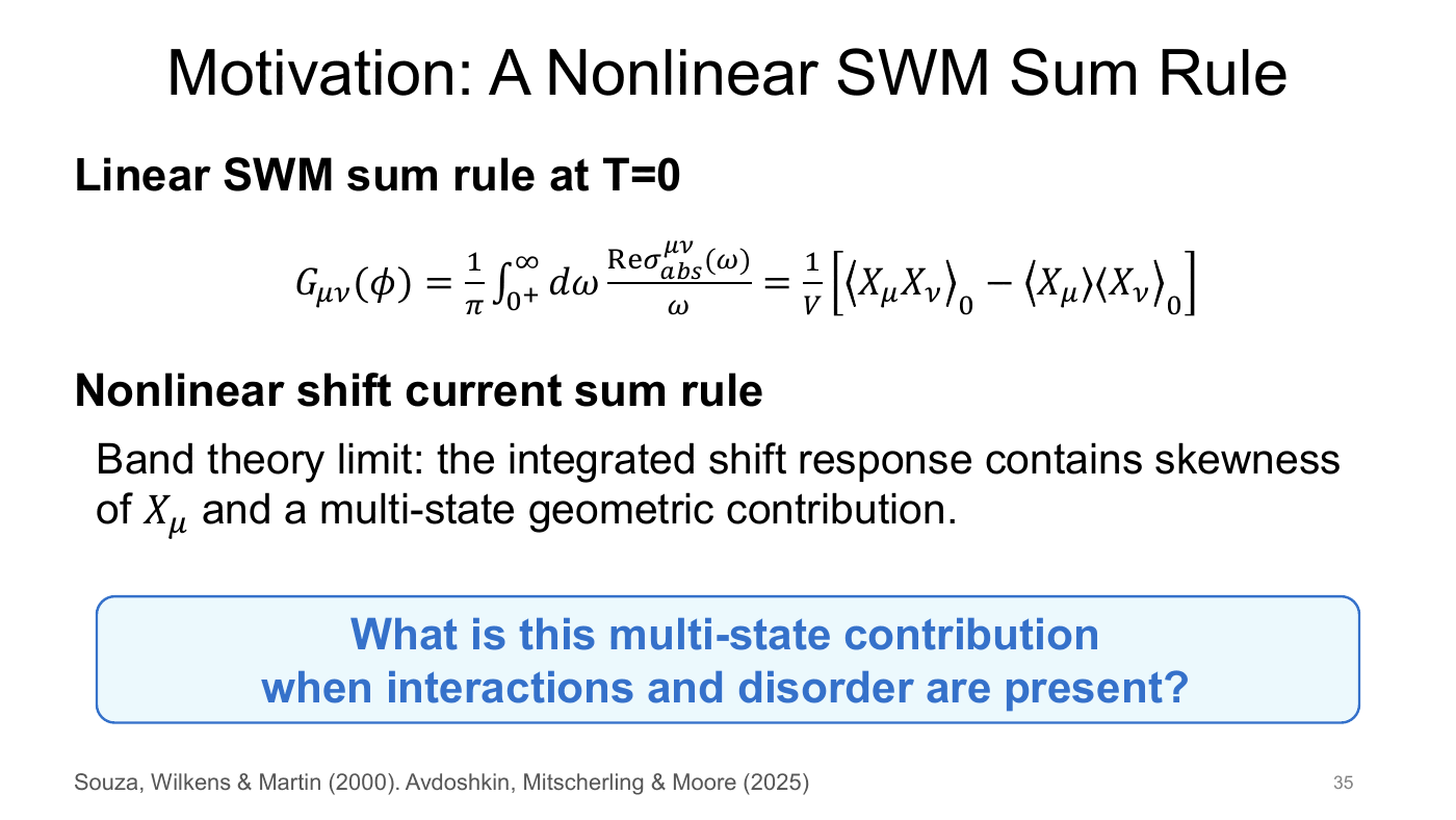
The goal is a sum rule for the shift part. At zero temperature, the linear SWM rule reads

$$ G_{\mu\nu}(\phi) = \frac1\pi\int_{0^+}^\infty\mathrm d\omega\,\frac{\mathrm{Re}\,\sigma^{\mu\nu}_{\text{abs}}(\omega)}{\omega} = \frac1V\big[\langle X_\mu X_\nu\rangle_0 - \langle X_\mu\rangle_0\langle X_\nu\rangle_0\big]. $$

In the band limit, the integrated shift response contains the skewness of $X_\mu$ plus a multi-state geometric contribution (Avdoshkin, Mitscherling & Moore 2025). What does that multi-state term become once interactions and disorder are present?

The many-body rectification sum rule

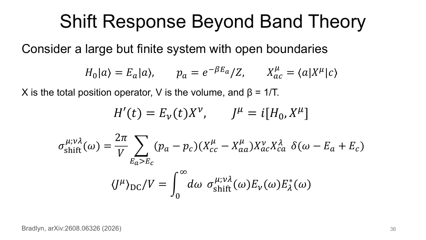
Consider a large but finite system with open boundaries: $H_0\lvert a\rangle = E_a\lvert a\rangle$, $p_a = e^{-\beta E_a}/Z$, with total position operator $X^\mu$ and matrix elements $X^\mu_{ac} = \langle a\rvert X^\mu\lvert c\rangle$. With $H'(t) = E_\nu(t)X^\nu$ and $J^\mu = i[H_0,X^\mu]$,

$$ \sigma^{\mu;\nu\lambda}_{\text{shift}}(\omega) = \frac{2\pi}{V}\sum_{E_a>E_c}(p_a-p_c)\,(X^\mu_{cc}-X^\mu_{aa})\,X^\nu_{ac}X^\lambda_{ca}\,\delta(\omega-E_a+E_c), $$

and the DC current is $\langle J^\mu\rangle_{\text{DC}}/V = \int_0^\infty\mathrm d\omega\,\sigma^{\mu;\nu\lambda}_{\text{shift}}(\omega)E_\nu(\omega)E^*_\lambda(\omega)$. The factor $X^\mu_{cc}-X^\mu_{aa}$ is the shift in position during the transition. Now let $\lvert0\rangle$ be the ground state, and define the position fluctuation and skewness,

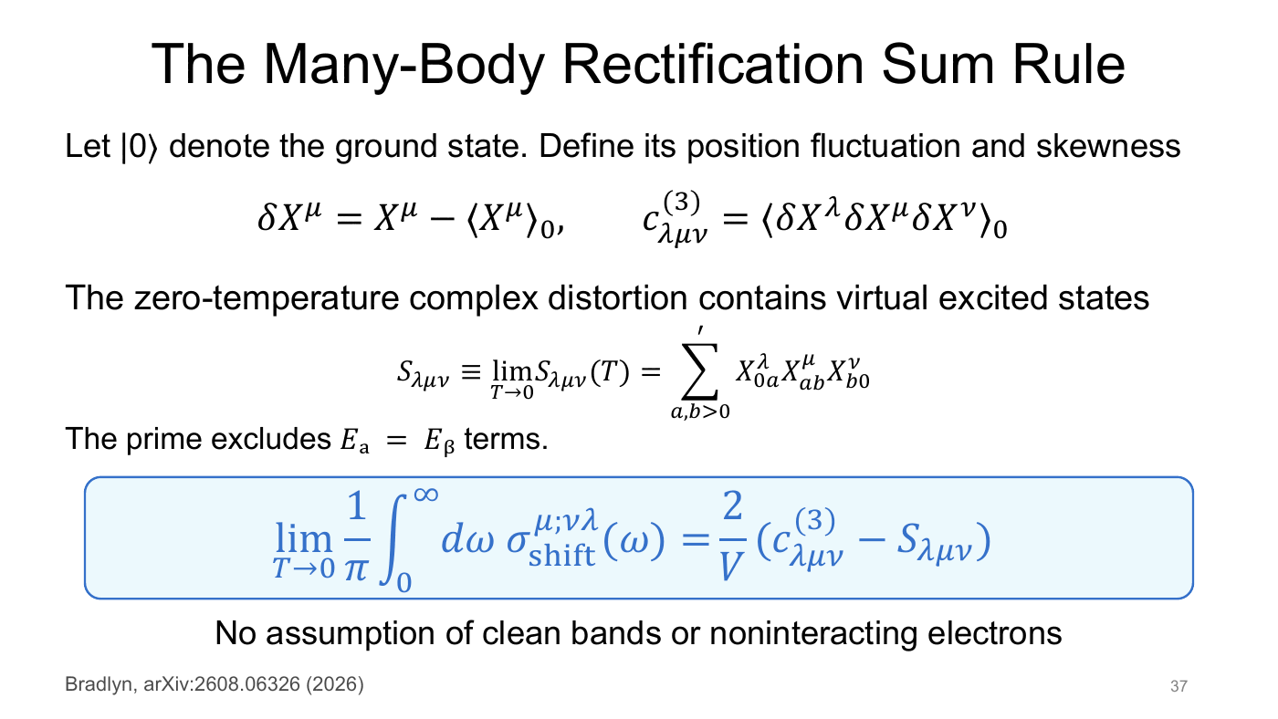
$$ \delta X^\mu = X^\mu - \langle X^\mu\rangle_0,\qquad c^{(3)}_{\lambda\mu\nu} = \langle\delta X^\lambda\,\delta X^\mu\,\delta X^\nu\rangle_0, $$

and the zero-temperature complex distortion

$$ S_{\lambda\mu\nu} \equiv \lim_{T\to0}S_{\lambda\mu\nu}(T) = {\sum_{a,b>0}}'\,X^\lambda_{0a}X^\mu_{ab}X^\nu_{b0}, $$

where the prime excludes terms with $E_a = E_b$. The sum rule is

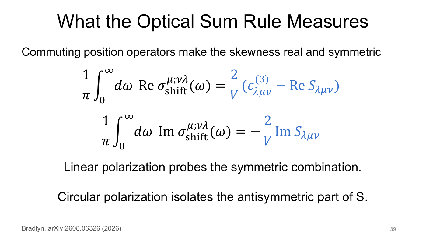
$$ \lim_{T\to0}\frac1\pi\int_0^\infty\mathrm d\omega\;\sigma^{\mu;\nu\lambda}_{\text{shift}}(\omega) = \frac2V\big(c^{(3)}_{\lambda\mu\nu} - S_{\lambda\mu\nu}\big). $$

It makes no assumption of clean bands or noninteracting electrons.

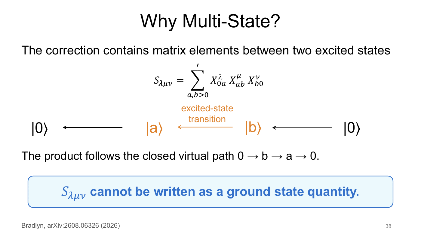
Why “multi-state”? $S_{\lambda\mu\nu}$ contains matrix elements between two excited states. The product traces a closed virtual path $0\to b\to a\to0$ that includes an excited-to-excited transition $b\to a$. So, unlike $c^{(3)}$, $S_{\lambda\mu\nu}$ cannot be written as a ground-state expectation value.

What an optical measurement sees. The position operators commute, so the skewness is real and totally symmetric. Splitting into real and imaginary parts gives

$$ \begin{aligned} \frac1\pi\int_0^\infty\mathrm d\omega\,\mathrm{Re}\,\sigma^{\mu;\nu\lambda}_{\text{shift}}(\omega) &= \frac2V\big(c^{(3)}_{\lambda\mu\nu} - \mathrm{Re}\,S_{\lambda\mu\nu}\big), \\ \frac1\pi\int_0^\infty\mathrm d\omega\,\mathrm{Im}\,\sigma^{\mu;\nu\lambda}_{\text{shift}}(\omega) &= -\frac2V\,\mathrm{Im}\,S_{\lambda\mu\nu}. \end{aligned} $$

Linearly polarized light probes the symmetric combination. Circularly polarized light isolates the antisymmetric part of $S$.

Where the distortion comes from: non-metricity

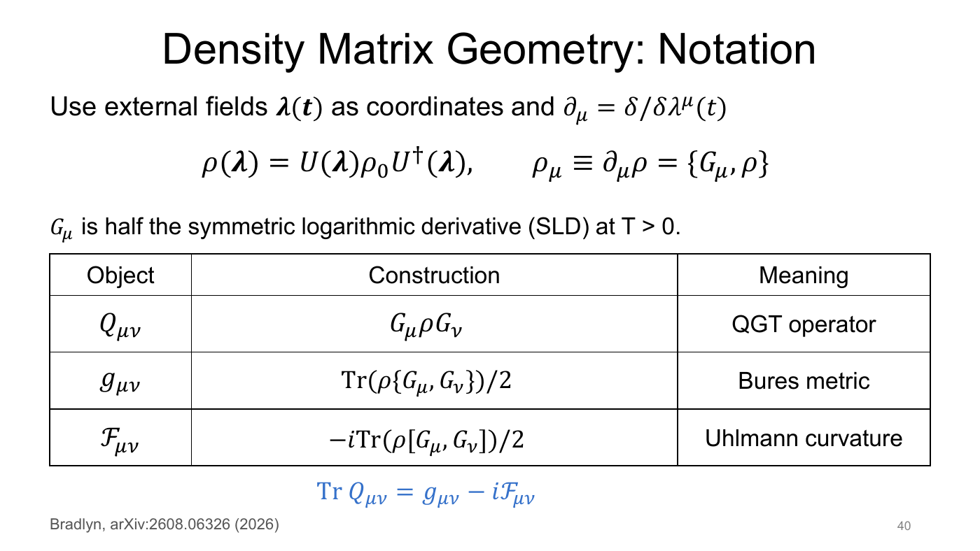
Notation. Use the external fields $\boldsymbol\lambda(t)$ as coordinates, with $\partial_\mu = \delta/\delta\lambda^\mu(t)$, and write $\rho(\boldsymbol\lambda) = U(\boldsymbol\lambda)\rho_0U^\dagger(\boldsymbol\lambda)$. The tangent vectors are $\rho_\mu \equiv \partial_\mu\rho = \{G_\mu,\rho\}$, where $G_\mu$ is half the symmetric logarithmic derivative (at $T>0$). From $G_\mu$ one builds three objects:

Object	Construction	Meaning
$Q_{\mu\nu}$	$G_\mu\,\rho\,G_\nu$	QGT operator
$g_{\mu\nu}$	$\tfrac12\operatorname{Tr}(\rho\{G_\mu,G_\nu\})$	Bures metric
$\mathcal F_{\mu\nu}$	$-\tfrac i2\operatorname{Tr}(\rho[G_\mu,G_\nu])$	Uhlmann curvature

The trace of the QGT operator gives $\operatorname{Tr}Q_{\mu\nu} = g_{\mu\nu} - i\mathcal F_{\mu\nu}$.

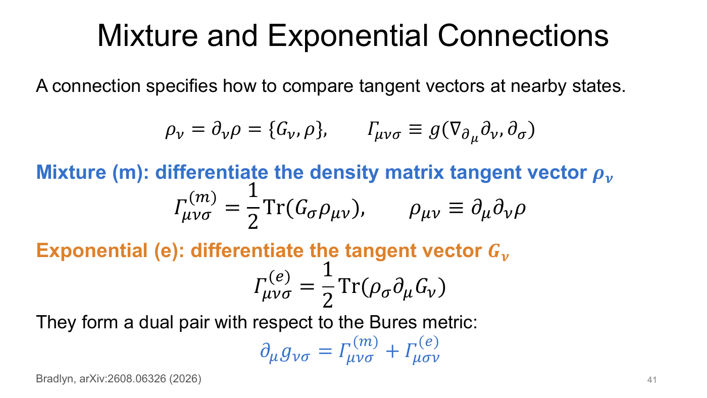
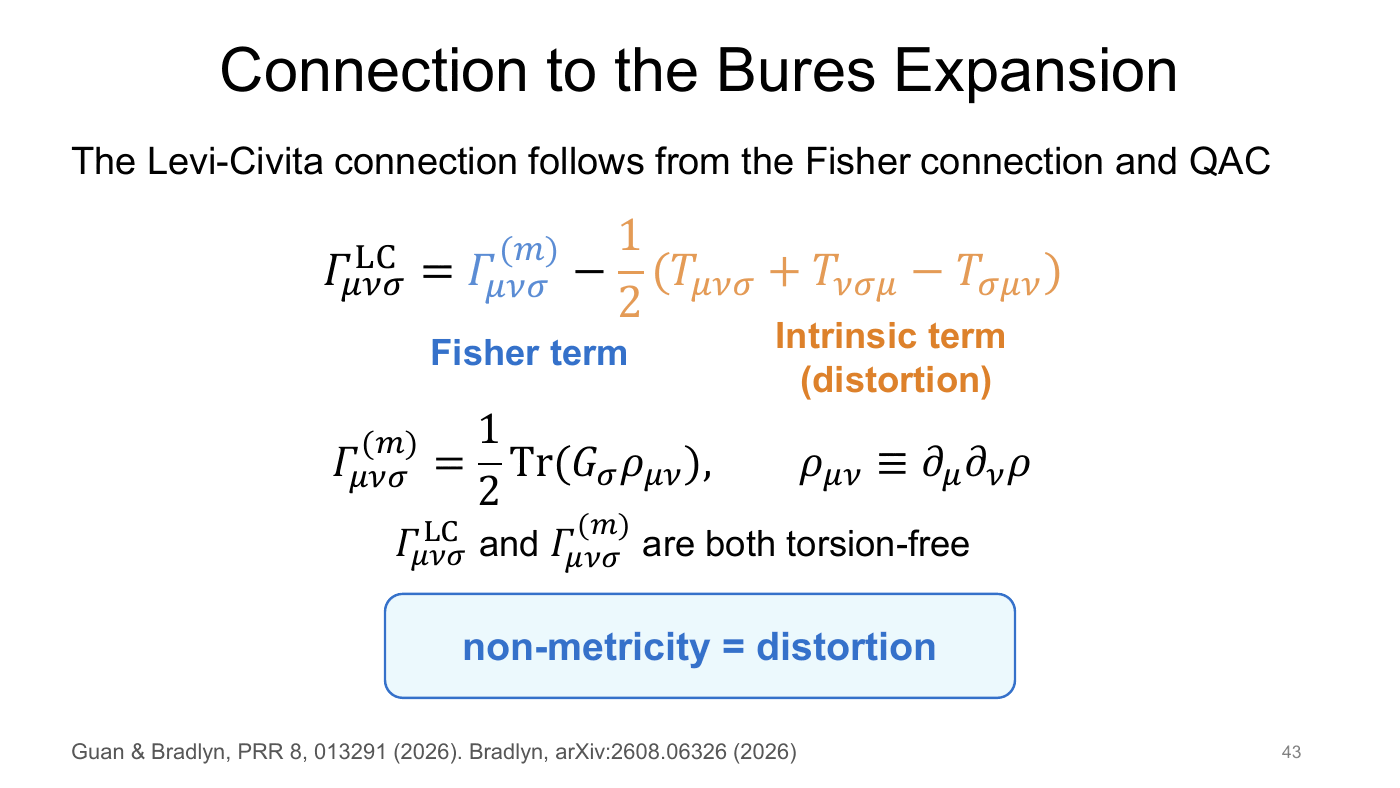
Mixture and exponential connections. A connection tells you how to compare tangent vectors at nearby states, $\Gamma_{\mu\nu\sigma} \equiv g(\nabla_{\partial_\mu}\partial_\nu,\partial_\sigma)$. There are two natural choices, depending on which representation of the tangent vector you differentiate:

$$ \Gamma^{(m)}_{\mu\nu\sigma} = \tfrac12\operatorname{Tr}(G_\sigma\,\rho_{\mu\nu}),\quad \rho_{\mu\nu}\equiv\partial_\mu\partial_\nu\rho \qquad\text{(mixture: differentiate } \rho_\nu\text{)}, $$$$ \Gamma^{(e)}_{\mu\nu\sigma} = \tfrac12\operatorname{Tr}(\rho_\sigma\,\partial_\mu G_\nu) \qquad\text{(exponential: differentiate } G_\nu\text{)}. $$

The two are dual with respect to the Bures metric, $\partial_\mu g_{\nu\sigma} = \Gamma^{(m)}_{\mu\nu\sigma} + \Gamma^{(e)}_{\mu\sigma\nu}$.

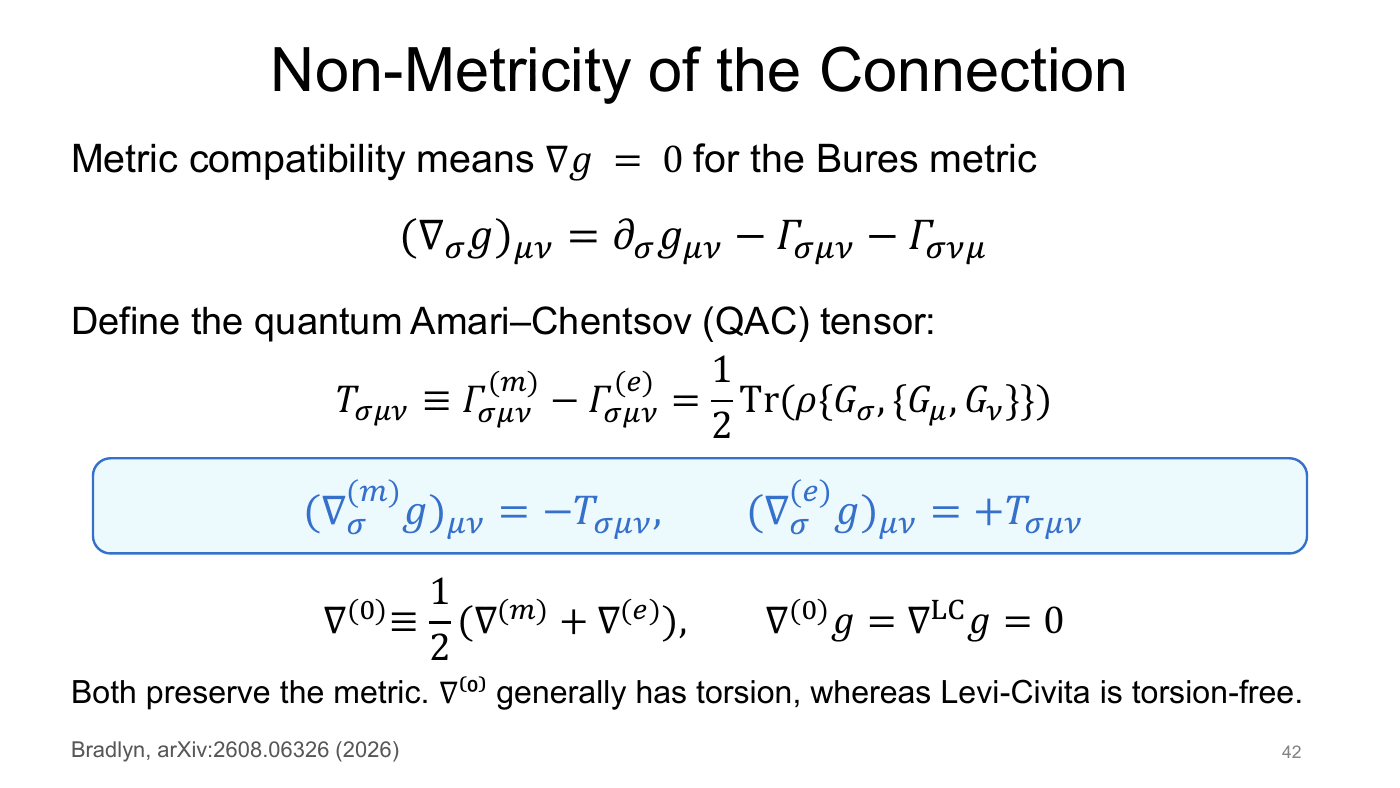
Non-metricity. Metric compatibility means $(\nabla_\sigma g)_{\mu\nu} = \partial_\sigma g_{\mu\nu} - \Gamma_{\sigma\mu\nu} - \Gamma_{\sigma\nu\mu} = 0$. Neither connection satisfies it. The failure is measured by the quantum Amari–Chentsov (QAC) tensor,

$$ \begin{aligned} T_{\sigma\mu\nu} &\equiv \Gamma^{(m)}_{\sigma\mu\nu} - \Gamma^{(e)}_{\sigma\mu\nu} = \tfrac12\operatorname{Tr}\big(\rho\{G_\sigma,\{G_\mu,G_\nu\}\}\big), \\ (\nabla^{(m)}_\sigma g)_{\mu\nu} &= -T_{\sigma\mu\nu},\qquad (\nabla^{(e)}_\sigma g)_{\mu\nu} = +T_{\sigma\mu\nu}. \end{aligned} $$

Their average $\nabla^{(0)} = \frac12(\nabla^{(m)}+\nabla^{(e)})$ preserves the metric, as does Levi-Civita. The difference is that $\nabla^{(0)}$ generally has torsion, while Levi-Civita is torsion-free.

Connection to the Bures expansion. The Levi-Civita connection is the mixture (“Fisher”) connection corrected by the QAC tensor:

$$ \Gamma^{\text{LC}}_{\mu\nu\sigma} = \underbrace{\Gamma^{(m)}_{\mu\nu\sigma}}_{\text{Fisher term}} - \underbrace{\tfrac12\big(T_{\mu\nu\sigma} + T_{\nu\sigma\mu} - T_{\sigma\mu\nu}\big)}_{\text{intrinsic term (distortion)}} . $$

Both $\Gamma^{\text{LC}}$ and $\Gamma^{(m)}$ are torsion-free, so their difference is pure distortion. This is the same Fisher/intrinsic split found in the Bures expansion of Part 4: non-metricity = distortion.

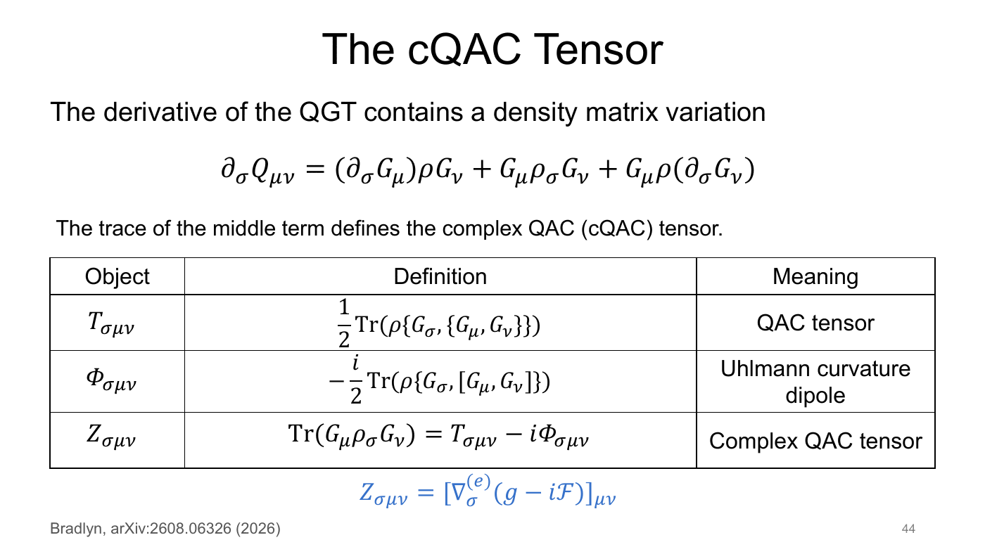
The complex version. Differentiating the QGT operator gives $\partial_\sigma Q_{\mu\nu} = (\partial_\sigma G_\mu)\rho G_\nu + G_\mu\rho_\sigma G_\nu + G_\mu\rho(\partial_\sigma G_\nu)$. The trace of the middle term defines the complex QAC tensor:

Object	Definition	Meaning
$T_{\sigma\mu\nu}$	$\tfrac12\operatorname{Tr}(\rho\{G_\sigma,\{G_\mu,G_\nu\}\})$	QAC tensor
$\Phi_{\sigma\mu\nu}$	$-\tfrac i2\operatorname{Tr}(\rho\{G_\sigma,[G_\mu,G_\nu]\})$	Uhlmann curvature dipole
$Z_{\sigma\mu\nu}$	$\operatorname{Tr}(G_\mu\rho_\sigma G_\nu) = T_{\sigma\mu\nu} - i\Phi_{\sigma\mu\nu}$	complex QAC tensor

The complex QAC tensor is itself a non-metricity, $Z_{\sigma\mu\nu} = [\nabla^{(e)}_\sigma(g - i\mathcal F)]_{\mu\nu}$.

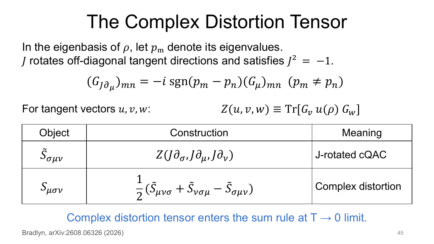
The complex distortion. Work in the eigenbasis of $\rho$, with eigenvalues $p_m$. Define a map $J$ that rotates off-diagonal tangent directions, with $J^2 = -1$: $(G_{J\partial_\mu})_{mn} = -i\,\mathrm{sgn}(p_m-p_n)\,(G_\mu)_{mn}$ for $p_m\ne p_n$. With $Z(u,v,w) \equiv \operatorname{Tr}[G_v\,u(\rho)\,G_w]$ for tangent vectors $u,v,w$, define the $J$-rotated cQAC tensor and the complex distortion:

$$ \tilde S_{\sigma\mu\nu} = Z(J\partial_\sigma,J\partial_\mu,J\partial_\nu),\qquad S_{\mu\sigma\nu} = \tfrac12\big(\tilde S_{\mu\nu\sigma} + \tilde S_{\nu\sigma\mu} - \tilde S_{\sigma\mu\nu}\big). $$

In the $T\to0$ limit, this is the $S_{\lambda\mu\nu}$ that enters the shift-current sum rule.

Summary

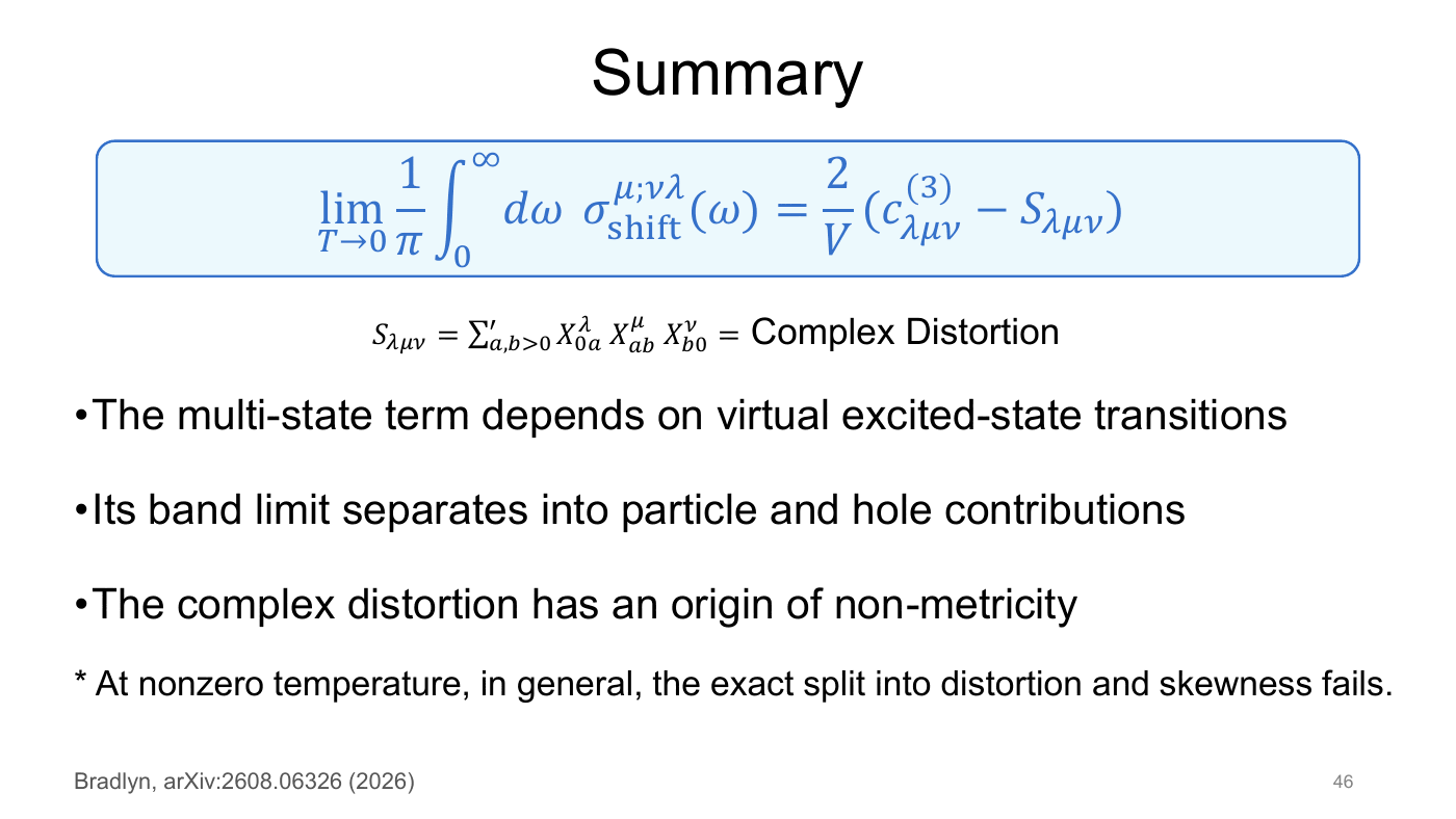
$$ \lim_{T\to0}\frac1\pi\int_0^\infty\mathrm d\omega\;\sigma^{\mu;\nu\lambda}_{\text{shift}}(\omega) = \frac2V\big(c^{(3)}_{\lambda\mu\nu} - S_{\lambda\mu\nu}\big), \qquad S_{\lambda\mu\nu} = {\sum_{a,b>0}}'\,X^\lambda_{0a}X^\mu_{ab}X^\nu_{b0}. $$

• The Bures distance between the equilibrium and driven density matrices gives a single geometric framework. At second order it defines a metric, which covers finite temperature, interactions and disorder, and arbitrary perturbing operators. At third order it defines a connection, which covers nonlinear response.
• The metric unifies the finite-$T$ SWM sum rule, the quantum Fisher information, and Fermi’s golden rule. At zero temperature the connection is the band-theory Christoffel symbol.
• The multi-state term in the shift-current sum rule depends on virtual excited-to-excited transitions. In the band limit it separates into particle and hole contributions, and it originates in the non-metricity of the mixture/exponential connections.
• Caveat: at nonzero temperature the exact split into skewness and distortion fails in general.

References

1. Y. Guan and B. Bradlyn, Phys. Rev. Research 8, 013291 (2026).
2. B. Bradlyn, “Multi-State Geometry of Density Matrices and Rectification Sum Rules,” arXiv:2608.06326 (2026).
3. B. Bradlyn and P. Abbamonte, Phys. Rev. B 110, 245132 (2024).
4. I. Souza, T. Wilkens, and R. M. Martin, Phys. Rev. B 62, 1666 (2000).
5. N. Marzari and D. Vanderbilt, Phys. Rev. B 56, 12847 (1997).
6. P. Hauke, M. Heyl, L. Tagliacozzo, and P. Zoller, Nat. Phys. 12, 778 (2016).
7. J. Ahn, G.-Y. Guo, N. Nagaosa, and A. Vishwanath, Nat. Phys. 18, 290 (2022).
8. H. Watanabe and M. Oshikawa, Phys. Rev. B 102, 165137 (2020).
9. S. Amari and H. Nagaoka, Methods of Information Geometry (AMS / Oxford University Press, 2000).