Generative Models: Variational Autoencoders and Diffusion Models

Presenter	Mengyao Zhang (Prof. Binghai Yan’s group, Penn State)
Date	September 21, 2026 · 4:30–6:00 PM
Location	Davey 339
Topic	Stat Mech in Machine Learning — generative models: VAEs and denoising diffusion
Notes	Handwritten, 6 pages (viewer and download below)

How do you draw a fresh sample from the distribution of natural images, when the only distributions you can sample directly are the uniform and the Gaussian? Both answers in this session start the same way. Draw a latent variable $z$ from a simple distribution, then learn a map that sends it to data. Training by maximum likelihood then runs into one obstacle: the posterior over the latent variable is intractable. The variational autoencoder handles it with one learned Gaussian posterior and a single decoding step, trained on the evidence lower bound (ELBO) with the reparameterization trick. The denoising diffusion probabilistic model (DDPM) has $T$ latent layers, and it fixes the approximate posterior to be a known noising process, so no encoder is learned at all. Its ELBO then collapses to a remarkably simple objective: predict the noise that was added. The handwritten notes carry every derivation, from the Gaussian-mixture M-step, through the closed-form Gaussian KL, to the DDPM posterior mean and sampling loop.

Part 0 — Where we left off: EM for a Gaussian mixture

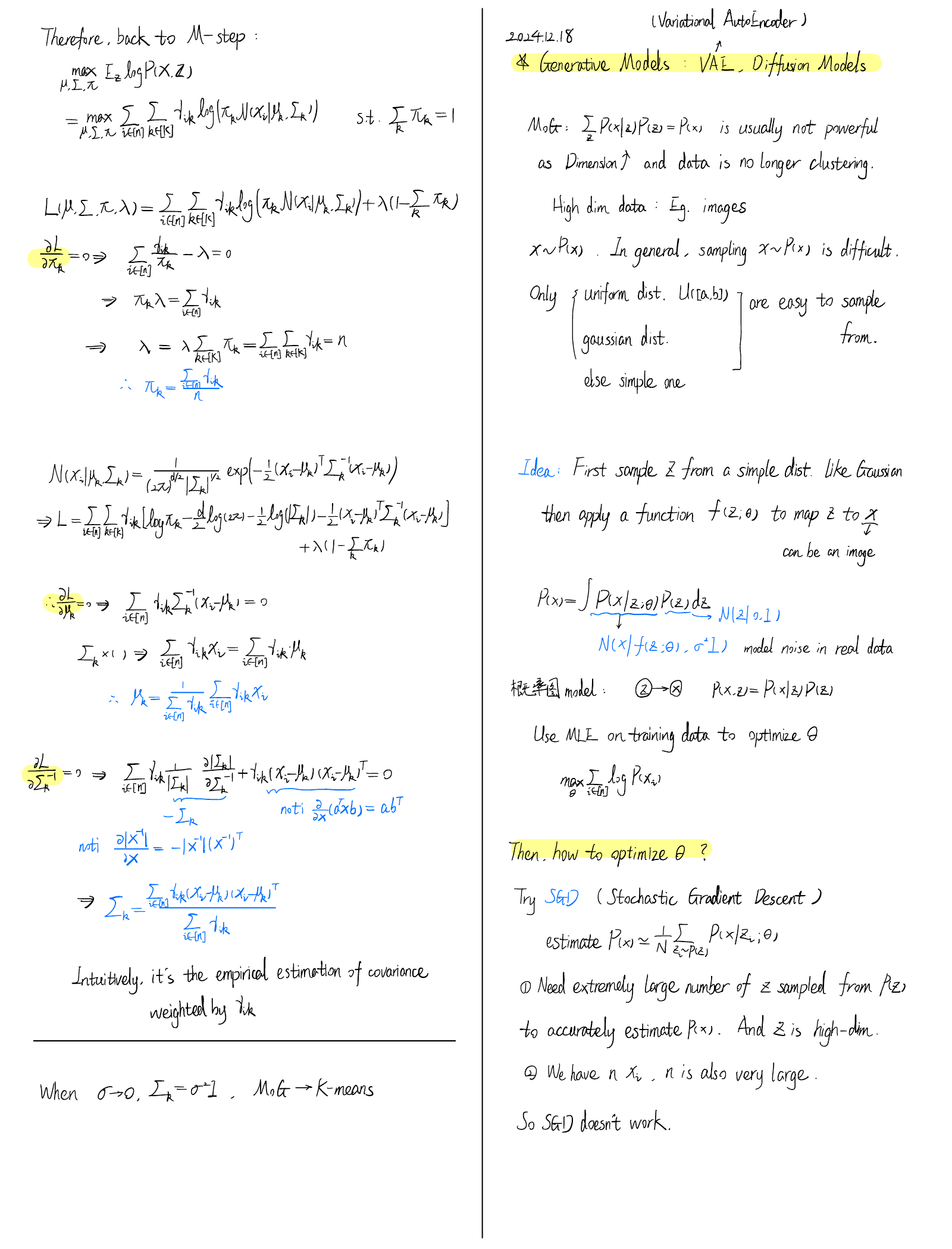
The notes open by finishing the previous session’s example. The Gaussian mixture model (MoG) has a discrete latent label $z\in[K]$, with $p(x) = \sum_k \pi_k\,\mathcal N(x\mid\mu_k,\Sigma_k)$. Let $\gamma_{ik} = p(z_i = k\mid x_i)$ be the responsibilities from the E-step. The M-step then maximizes the expected complete-data log-likelihood under the constraint $\sum_k\pi_k = 1$:

$$ \mathcal L(\mu,\Sigma,\pi,\lambda) = \sum_{i\in[n]}\sum_{k\in[K]} \gamma_{ik} \log\!\big(\pi_k\,\mathcal N(x_i\mid\mu_k,\Sigma_k)\big) + \lambda\Big(1-\sum_k\pi_k\Big). $$

Setting the derivatives to zero gives three closed-form updates:

$$ \pi_k = \frac{1}{n}\sum_{i}\gamma_{ik},\qquad \mu_k = \frac{\sum_i \gamma_{ik}\,x_i}{\sum_i\gamma_{ik}},\qquad \Sigma_k = \frac{\sum_i \gamma_{ik}\,(x_i-\mu_k)(x_i-\mu_k)^{\mathsf T}}{\sum_i\gamma_{ik}}. $$

For $\pi_k$, the multiplier comes out as $\lambda = \sum_{i,k}\gamma_{ik} = n$. For $\Sigma_k$, it is easiest to differentiate with respect to $\Sigma_k^{-1}$, using $\partial_X\,a^{\mathsf T}Xb = ab^{\mathsf T}$ and $\partial_X \lvert X^{-1}\rvert = -\lvert X^{-1}\rvert\,(X^{-1})^{\mathsf T}$. Each update is an empirical estimate (weight, mean, covariance) weighted by the responsibilities. In the limit $\Sigma_k = \sigma^2 I$ with $\sigma\to 0$, the responsibilities become hard assignments, and MoG reduces to $K$-means.

Part 1 — Why generative modelling is hard

A mixture $p(x) = \sum_z p(x\mid z)p(z)$ is not expressive enough once the dimension grows and the data stop forming clusters. Images are the standard example. In general, drawing $x\sim p(x)$ is hard. The distributions we can sample directly are the uniform $U[a,b]$, the Gaussian, and a few other simple ones.

Idea. First sample $z$ from a simple distribution such as a Gaussian. Then apply a learned function $f(z;\theta)$ that maps $z$ to $x$, for example an image:

$$ \begin{aligned} p(x) &= \int p(x\mid z;\theta)\,p(z)\,\mathrm dz, \\ p(z) &= \mathcal N(z\mid 0, I),\qquad p(x\mid z;\theta) = \mathcal N\!\big(x\mid f(z;\theta),\,\sigma^2 I\big). \end{aligned} $$

The Gaussian around $f(z;\theta)$ models noise in real data. The graphical model is simply $z\to x$, with $p(x,z) = p(x\mid z)\,p(z)$. Training is maximum likelihood on the data, $\max_\theta \sum_{i\in[n]}\log p(x_i)$.

How do we optimize $\theta$?

• Plain SGD would need a Monte Carlo estimate of the marginal, $p(x)\approx \frac1N\sum_{z\sim p(z)} p(x\mid z;\theta)$. Two things go wrong. Because $z$ is high-dimensional, $N$ has to be enormous before the estimate is accurate. And the number of data points $n$ is also large. So this fails.
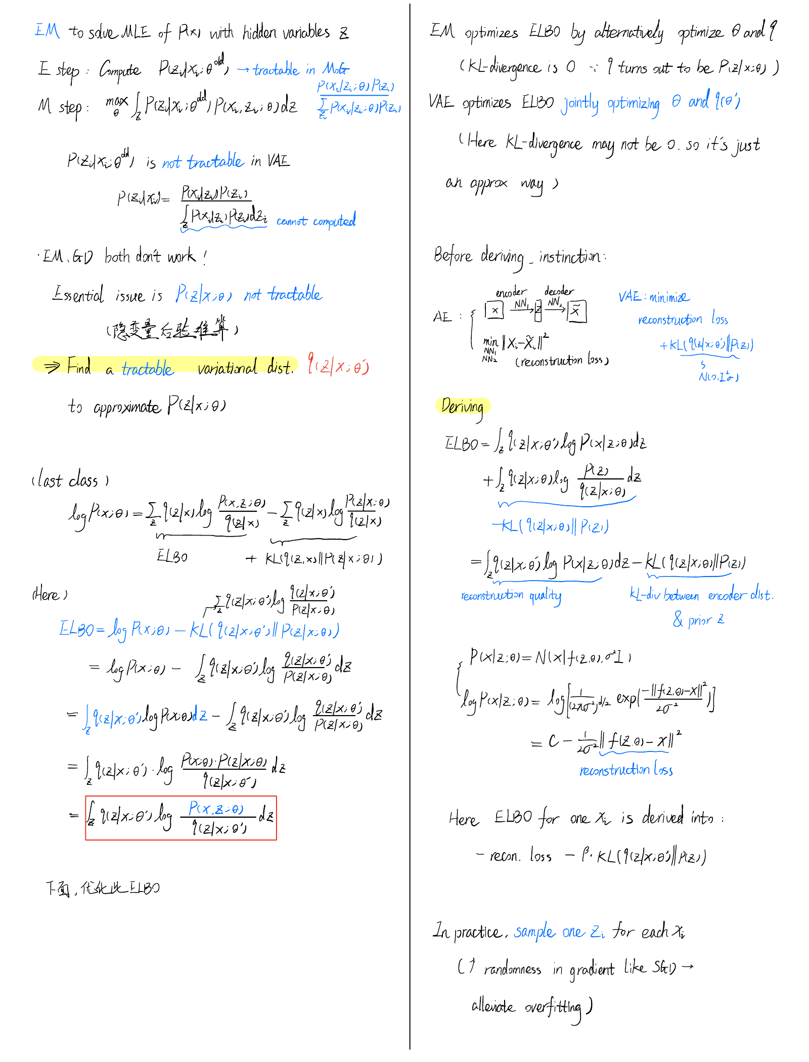
• EM would alternate an E-step, computing $p(z\mid x_i;\theta^{\text{old}})$, with an M-step, $\max_\theta\int p(z\mid x_i;\theta^{\text{old}})\log p(x_i,z;\theta)\,\mathrm dz$. For MoG the E-step is tractable. Here it is not, because the posterior $$ p(z\mid x_i) = \frac{p(x_i\mid z)\,p(z)}{\int p(x_i\mid z)\,p(z)\,\mathrm dz} $$ has an evidence integral in the denominator that we cannot compute.

So EM and gradient descent both fail, and for the same reason: the posterior $p(z\mid x;\theta)$ over the latent variable is intractable. The way out is to find a tractable variational distribution $q(z\mid x;\theta')$ that approximates it.

Part 2 — The ELBO

For any $q$, the log-evidence splits into two parts:

$$ \log p(x;\theta) = \underbrace{\int q(z\mid x)\log\frac{p(x,z;\theta)}{q(z\mid x)}\,\mathrm dz}_{\text{ELBO}} \;+\; \mathrm{KL}\big(q(z\mid x)\,\big\Vert\, p(z\mid x;\theta)\big). $$

Read the other way round, the ELBO is the log-evidence minus the approximation error:

$$ \begin{aligned} \mathrm{ELBO} &= \log p(x;\theta) - \mathrm{KL}\big(q(z\mid x;\theta')\,\Vert\,p(z\mid x;\theta)\big) \\ &= \int q(z\mid x;\theta')\,\log\frac{p(x,z;\theta)}{q(z\mid x;\theta')}\,\mathrm dz . \end{aligned} $$

Since $\mathrm{KL}\ge0$, the ELBO is a lower bound on $\log p(x;\theta)$. Two algorithms maximize it in different ways:

• EM maximizes the ELBO by optimizing $\theta$ and $q$ alternately. The E-step sets $q$ to the exact posterior $p(z\mid x;\theta)$, so the KL term is exactly zero.
• The VAE maximizes the ELBO by optimizing $\theta$ and the variational parameters $\theta'$ jointly. Here the KL term need not vanish, so the result is an approximation.

Part 3 — The variational autoencoder

Intuition first. A plain autoencoder has two networks. An encoder (NN$_1$) maps $x$ to a code $z$, and a decoder (NN$_2$) maps $z$ back to $\tilde x$. Both are trained on the reconstruction loss $\min\lVert x-\tilde x\rVert^2$. A VAE minimizes the same reconstruction loss plus a KL term that pulls the encoder’s distribution towards the prior $\mathcal N(0,I)$.

Derivation. Splitting $p(x,z) = p(x\mid z)\,p(z)$ inside the ELBO gives

$$ \mathrm{ELBO} = \underbrace{\int q(z\mid x;\theta')\log p(x\mid z;\theta)\,\mathrm dz}_{\text{reconstruction quality}} \;-\; \underbrace{\mathrm{KL}\big(q(z\mid x;\theta')\,\Vert\,p(z)\big)}_{\text{encoder vs. prior}} . $$

With the Gaussian decoder, $\log p(x\mid z;\theta) = C - \frac{1}{2\sigma^2}\lVert f(z;\theta)-x\rVert^2$, which is a reconstruction loss. For one data point, the ELBO is therefore $-(\text{recon. loss}) - \beta\,\mathrm{KL}\big(q(z\mid x_i;\theta')\,\Vert\,p(z)\big)$. The weight $\beta$ absorbs the $2\sigma^2$. In practice one samples a single $z_i$ for each $x_i$. The extra noise in the gradient acts like SGD noise and helps against overfitting.

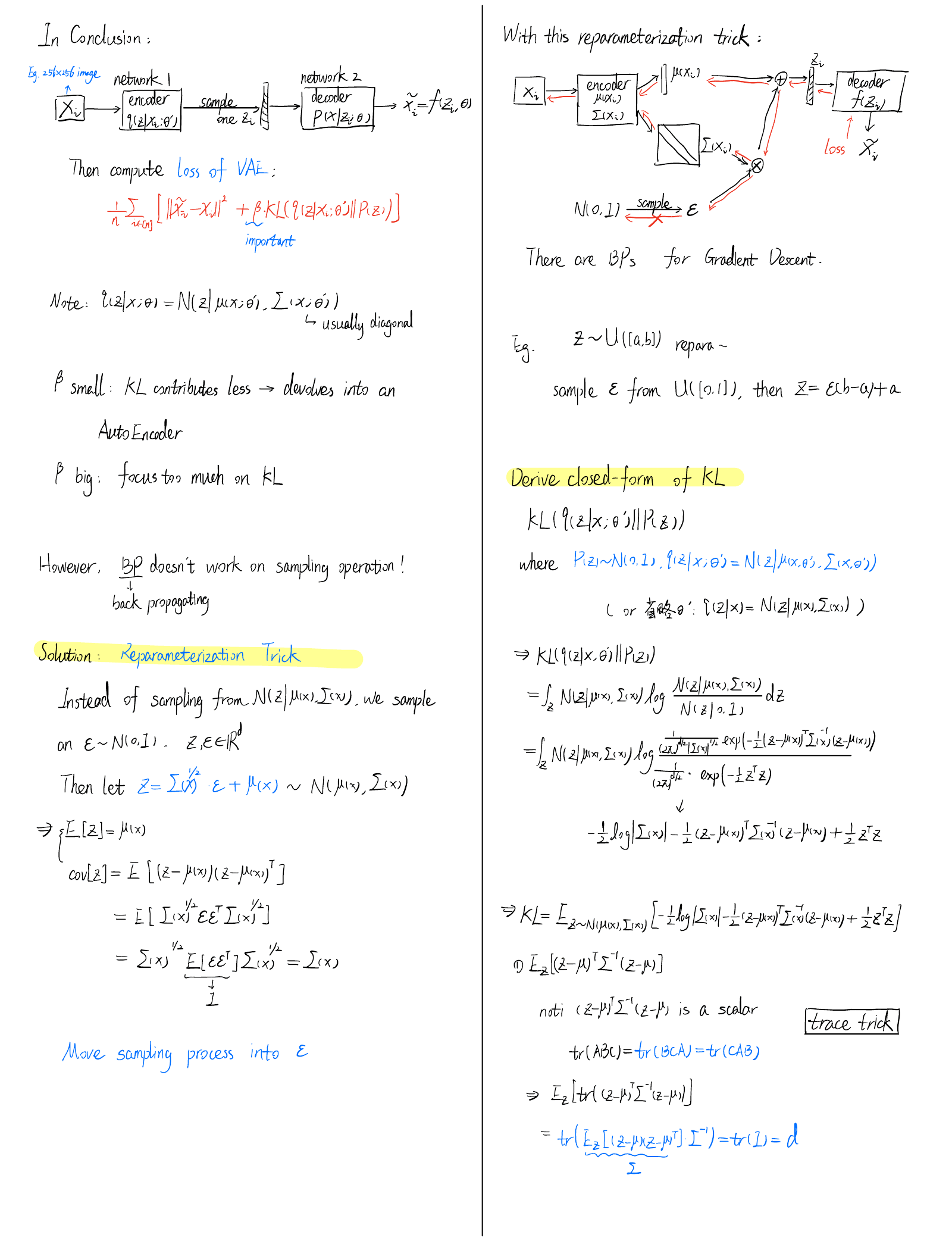
The whole pipeline. An input $x_i$ (say a $256\times256$ image) goes into the encoder $q(z\mid x_i;\theta')$. One $z_i$ is sampled from it and passed to the decoder $p(x\mid z_i;\theta)$, which outputs $\tilde x_i = f(z_i;\theta)$. The loss is

$$ \frac1n\sum_{i\in[n]}\Big[\lVert\tilde x_i - x_i\rVert^2 + \beta\, \mathrm{KL}\big(q(z\mid x_i;\theta')\,\Vert\,p(z)\big)\Big], $$

with encoder $q(z\mid x;\theta') = \mathcal N\big(z\mid \mu(x;\theta'),\,\Sigma(x;\theta')\big)$, where $\Sigma$ is usually diagonal. $\beta$ matters. If it is small, the KL term contributes little, and the model devolves into an ordinary autoencoder. If it is large, the model focuses too much on matching the prior, at the expense of reconstruction.

The reparameterization trick

Backpropagation cannot pass through a sampling operation. The fix is to move the randomness into an auxiliary variable. Draw $\varepsilon\sim\mathcal N(0,I)$ with $z,\varepsilon\in\mathbb R^d$, and set

$$ z = \Sigma(x)^{1/2}\,\varepsilon + \mu(x) \;\sim\; \mathcal N\big(\mu(x),\Sigma(x)\big). $$

It is easy to check that this has the right mean and covariance: $\mathbb E[z] = \mu(x)$, and $\operatorname{cov}[z] = \Sigma^{1/2}\,\mathbb E[\varepsilon\varepsilon^{\mathsf T}]\,\Sigma^{1/2} = \Sigma(x)$. Now the sampling happens at a leaf of the computational graph. Gradients reach the encoder through $\mu(x)$ and $\Sigma(x)$, and nothing ever differentiates through the draw of $\varepsilon$. The same idea works for other distributions. For example, $z\sim U[a,b]$ becomes $\varepsilon\sim U[0,1]$ with $z = \varepsilon(b-a)+a$.

Closed-form KL to a standard normal

With $q = \mathcal N(\mu,\Sigma)$ and $p(z) = \mathcal N(0,I)$ (dropping the $x$ and $\theta'$ labels), the log-ratio of densities is

$$ \log\frac{\mathcal N(z\mid\mu,\Sigma)}{\mathcal N(z\mid0,I)} = -\tfrac12\log\lvert\Sigma\rvert - \tfrac12(z-\mu)^{\mathsf T}\Sigma^{-1}(z-\mu) + \tfrac12 z^{\mathsf T}z . $$

Both quadratic terms can be averaged over $z\sim q$ with the trace trick, $\operatorname{tr}(ABC)=\operatorname{tr}(BCA)$:

$$ \begin{aligned} \mathbb E_z\big[(z-\mu)^{\mathsf T}\Sigma^{-1}(z-\mu)\big] &= \operatorname{tr}\!\big(\mathbb E_z[(z-\mu)(z-\mu)^{\mathsf T}]\,\Sigma^{-1}\big) = \operatorname{tr} I = d, \\ \mathbb E_z[z^{\mathsf T}z] &= \operatorname{tr}\Sigma + \mu^{\mathsf T}\mu . \end{aligned} $$

Putting these together,

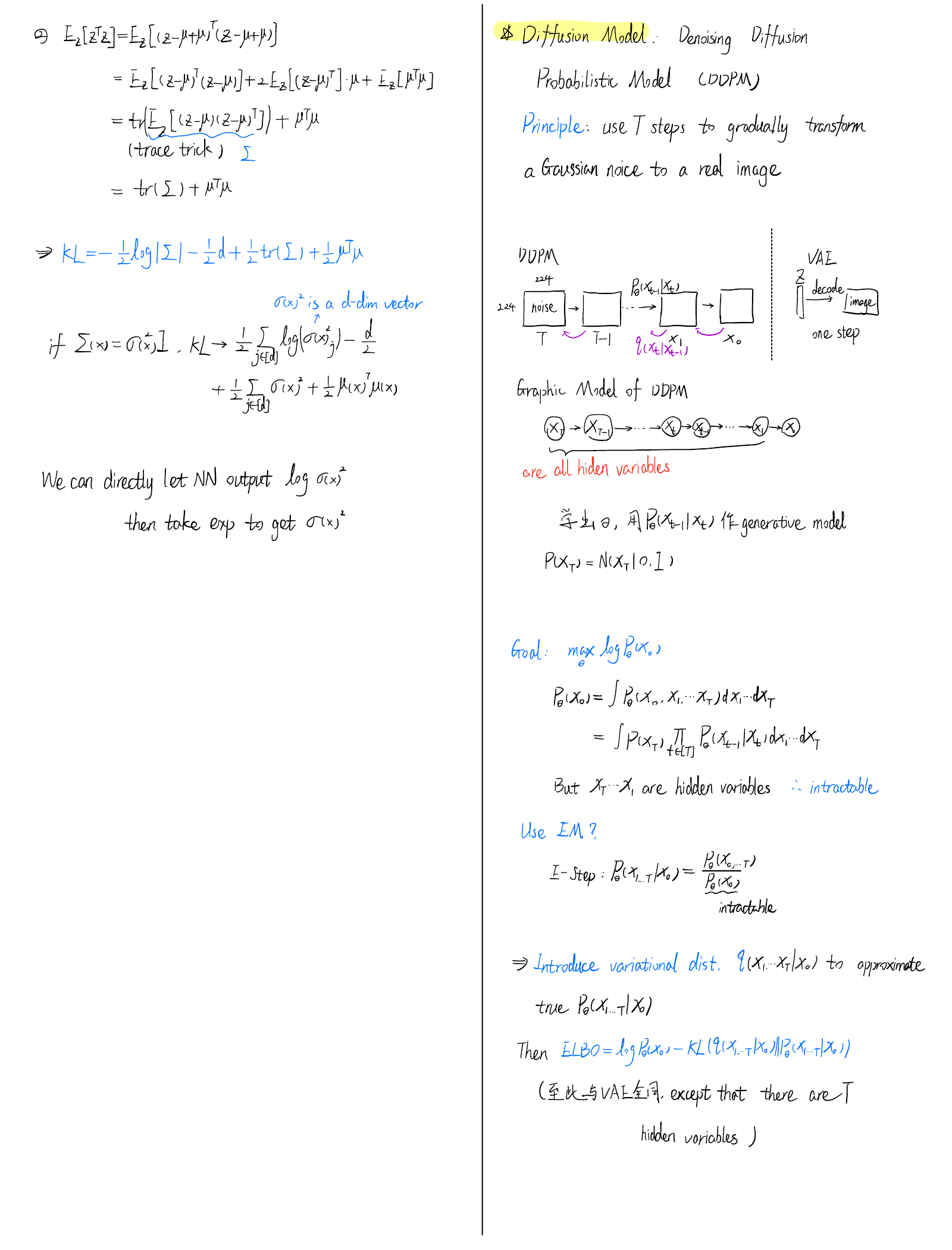
$$ \mathrm{KL}\big(\mathcal N(\mu,\Sigma)\,\Vert\,\mathcal N(0,I)\big) = -\tfrac12\log\lvert\Sigma\rvert - \tfrac d2 + \tfrac12\operatorname{tr}\Sigma + \tfrac12\mu^{\mathsf T}\mu . $$

For a diagonal covariance $\Sigma(x) = \operatorname{diag}\sigma(x)^2$, where $\sigma(x)^2$ is a $d$-dimensional vector, this becomes

$$ \mathrm{KL} = \frac12\sum_{j\in[d]}\Big(\sigma_j(x)^2 + \mu_j(x)^2 - \log\sigma_j(x)^2 - 1\Big). $$

In practice, the network outputs $\log\sigma(x)^2$ and exponentiates it. That keeps the variance positive without any constraint.

Part 4 — Denoising diffusion probabilistic models

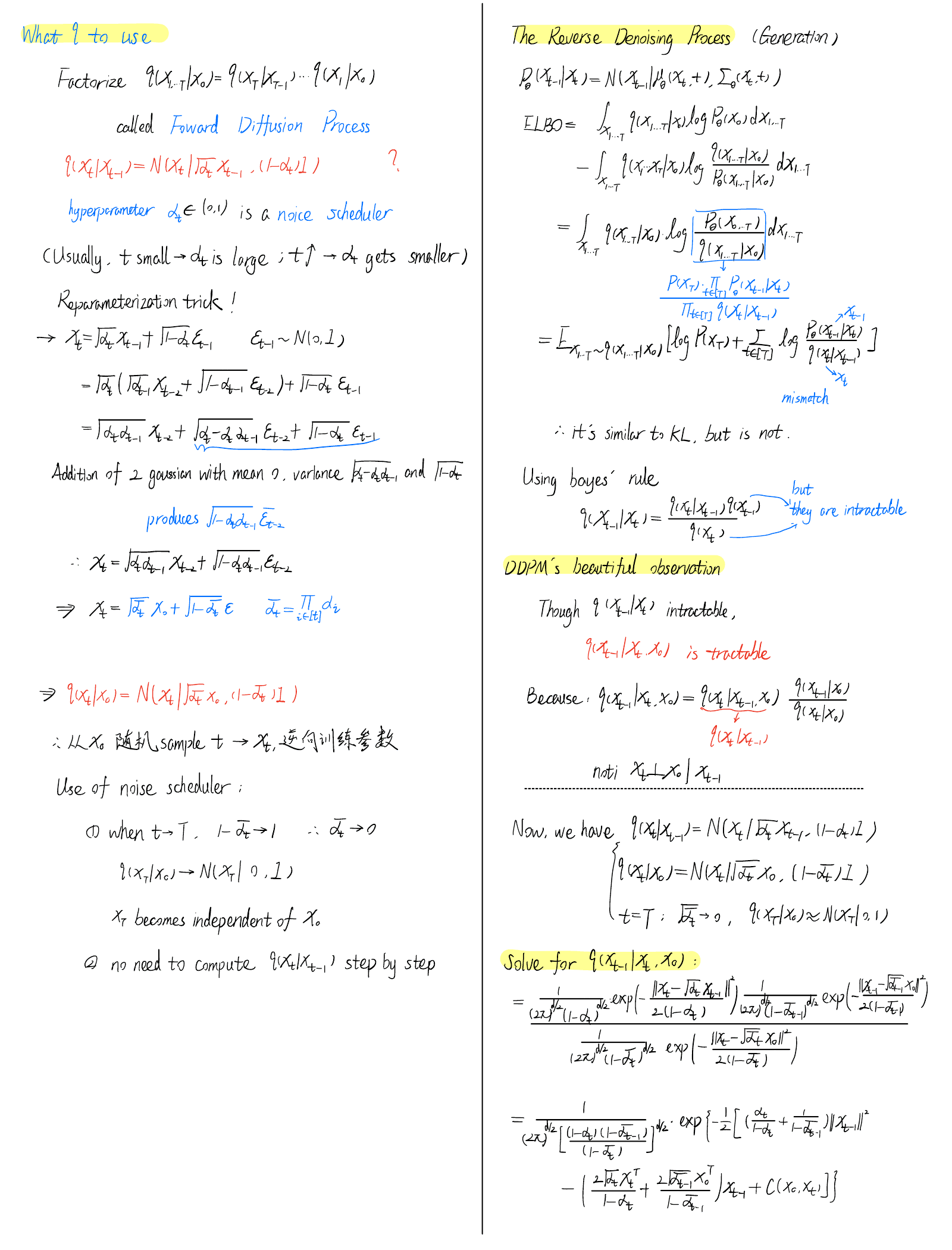
Principle. Use $T$ steps to gradually transform Gaussian noise into a real image. A VAE decodes $z$ to an image in one step. A DDPM runs a chain $x_T\to x_{T-1}\to\cdots\to x_1\to x_0$ in which every intermediate $x_t$ has the size of the image (e.g. $224\times224$). All of $x_T,\dots,x_1$ are hidden variables. The generative model is the learned reverse chain, with a fixed starting point:

$$ p(x_T) = \mathcal N(x_T\mid0,I),\qquad p_\theta(x_{t-1}\mid x_t) = \mathcal N\big(x_{t-1}\mid\mu_\theta(x_t,t),\,\Sigma_\theta(x_t,t)\big). $$

Goal. Maximize $\log p_\theta(x_0)$, where

$$ p_\theta(x_0) = \int p(x_T)\prod_{t\in[T]}p_\theta(x_{t-1}\mid x_t)\,\mathrm dx_1\cdots\mathrm dx_T . $$

This integral runs over all the hidden variables, so it is intractable. EM does not help either, since the E-step posterior $p_\theta(x_{1:T}\mid x_0) = p_\theta(x_{0:T})/p_\theta(x_0)$ contains the same intractable denominator. So, as before, introduce a variational distribution $q(x_{1:T}\mid x_0)$:

$$ \mathrm{ELBO} = \log p_\theta(x_0) - \mathrm{KL}\big(q(x_{1:T}\mid x_0)\,\Vert\,p_\theta(x_{1:T}\mid x_0)\big). $$

Up to this point, everything is identical to the VAE, except that there are $T$ hidden variables instead of one.

Which $q$? The forward diffusion process

Here DDPM departs from the VAE. The posterior $q$ is not learned. It is fixed to a Markov chain that adds noise, called the forward diffusion process:

$$ q(x_{1:T}\mid x_0) = \prod_{t=1}^T q(x_t\mid x_{t-1}),\qquad q(x_t\mid x_{t-1}) = \mathcal N\big(x_t\mid\sqrt{\alpha_t}\,x_{t-1},\,(1-\alpha_t)I\big). $$

The hyperparameters $\alpha_t\in(0,1)$ form the noise schedule. Usually $\alpha_t$ is close to 1 for small $t$ and decreases as $t$ grows. Writing each step with the reparameterization trick, $x_t = \sqrt{\alpha_t}\,x_{t-1} + \sqrt{1-\alpha_t}\,\varepsilon_{t-1}$, and unrolling one step gives

$$ x_t = \sqrt{\alpha_t\alpha_{t-1}}\,x_{t-2} + \sqrt{\alpha_t-\alpha_t\alpha_{t-1}}\,\varepsilon_{t-2} + \sqrt{1-\alpha_t}\,\varepsilon_{t-1}. $$

The last two terms are independent zero-mean Gaussians, with variances $\alpha_t-\alpha_t\alpha_{t-1}$ and $1-\alpha_t$. Their sum is therefore a single Gaussian with variance $1-\alpha_t\alpha_{t-1}$. Repeating this all the way down to $x_0$ gives a closed form:

$$ \begin{aligned} x_t &= \sqrt{\bar\alpha_t}\,x_0 + \sqrt{1-\bar\alpha_t}\,\varepsilon,\qquad \bar\alpha_t = \prod_{i\le t}\alpha_i, \\ q(x_t\mid x_0) &= \mathcal N\big(x_t\mid\sqrt{\bar\alpha_t}\,x_0,\,(1-\bar\alpha_t)I\big). \end{aligned} $$

This closed form does two jobs. (1) As $t\to T$ we have $\bar\alpha_T\to0$, so $q(x_T\mid x_0)\to\mathcal N(0,I)$ and $x_T$ becomes independent of $x_0$. The forward process ends at the same distribution the generative model starts from. (2) Training never has to run the chain step by step. You take $x_0$, pick a random $t$, jump straight to $x_t$, and train the reverse step there.

The reverse (generation) process and the ELBO

Substituting the factorized $q$ and $p_\theta$ into the ELBO gives

$$ \mathrm{ELBO} = \mathbb E_{x_{1:T}\sim q(x_{1:T}\mid x_0)}\Big[\log p(x_T) + \sum_{t\in[T]}\log\frac{p_\theta(x_{t-1}\mid x_t)}{q(x_t\mid x_{t-1})}\Big]. $$

Each term looks like a KL divergence, but it is not one. The numerator is a distribution over $x_{t-1}$ given $x_t$. The denominator runs the other way, over $x_t$ given $x_{t-1}$. Bayes’ rule would reverse the denominator, $q(x_{t-1}\mid x_t) = q(x_t\mid x_{t-1})\,q(x_{t-1})/q(x_t)$, but the marginals $q(x_{t-1})$ and $q(x_t)$ are intractable.

DDPM’s key observation. $q(x_{t-1}\mid x_t)$ is intractable, but $q(x_{t-1}\mid x_t, x_0)$ is tractable. By Bayes’ rule,

$$ q(x_{t-1}\mid x_t,x_0) = \frac{q(x_t\mid x_{t-1},x_0)\,q(x_{t-1}\mid x_0)}{q(x_t\mid x_0)}, $$

and $q(x_t\mid x_{t-1},x_0) = q(x_t\mid x_{t-1})$ because $x_t\perp x_0\mid x_{t-1}$ (the forward chain is Markov). All three factors are Gaussians that we already know. Collecting the terms quadratic and linear in $x_{t-1}$ in the exponent, and completing the square, gives

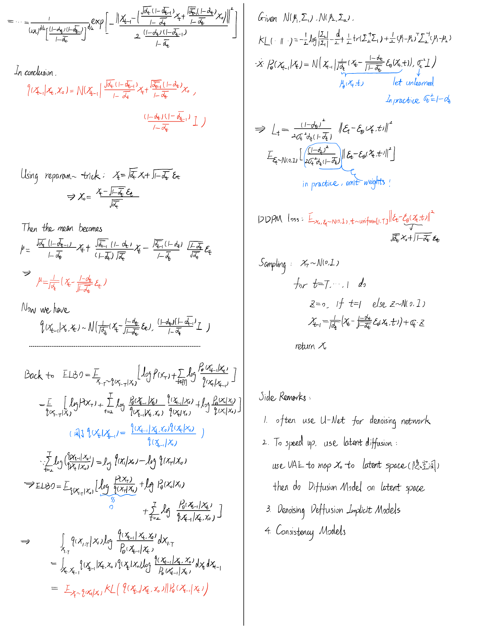
$$ \begin{aligned} q(x_{t-1}\mid x_t,x_0) &= \mathcal N\big(x_{t-1}\mid \tilde\mu_t(x_t,x_0),\,\tilde\beta_t I\big), \\ \tilde\mu_t(x_t,x_0) &= \frac{\sqrt{\alpha_t}(1-\bar\alpha_{t-1})}{1-\bar\alpha_t}\,x_t + \frac{\sqrt{\bar\alpha_{t-1}}(1-\alpha_t)}{1-\bar\alpha_t}\,x_0, \\ \tilde\beta_t &= \frac{(1-\alpha_t)(1-\bar\alpha_{t-1})}{1-\bar\alpha_t}. \end{aligned} $$

Next, eliminate $x_0$ from $\tilde\mu_t$ using $x_0 = (x_t-\sqrt{1-\bar\alpha_t}\,\varepsilon_t)/\sqrt{\bar\alpha_t}$. The mean then depends only on $x_t$ and the noise:

$$ \tilde\mu_t = \frac{1}{\sqrt{\alpha_t}}\Big(x_t - \frac{1-\alpha_t}{\sqrt{1-\bar\alpha_t}}\,\varepsilon_t\Big). $$

Back to the ELBO. Rewrite each forward factor for $t\ge2$ with Bayes’ rule, conditioning on $x_0$: $q(x_t\mid x_{t-1}) = q(x_{t-1}\mid x_t,x_0)\,q(x_t\mid x_0)/q(x_{t-1}\mid x_0)$. The ratios $q(x_{t-1}\mid x_0)/q(x_t\mid x_0)$ telescope to $q(x_1\mid x_0)/q(x_T\mid x_0)$, which leaves

$$ \mathrm{ELBO} = \mathbb E_{q}\Big[\underbrace{\log\frac{p(x_T)}{q(x_T\mid x_0)}}_{\approx\,0} + \log p_\theta(x_0\mid x_1) + \sum_{t=2}^T\log\frac{p_\theta(x_{t-1}\mid x_t)}{q(x_{t-1}\mid x_t,x_0)}\Big]. $$

The first term has no parameters, and it vanishes as $q(x_T\mid x_0)\to\mathcal N(0,I)$. Each term in the sum is now a genuine KL divergence between two distributions over $x_{t-1}$:

$$ -\,\mathbb E_{x_t\sim q(x_t\mid x_0)}\,\mathrm{KL}\big(q(x_{t-1}\mid x_t,x_0)\,\Vert\,p_\theta(x_{t-1}\mid x_t)\big). $$

From KL to “predict the noise”

The KL between two Gaussians is

$$ \begin{aligned} \mathrm{KL}\big(\mathcal N(\mu_1,\Sigma_1)\,\Vert\,\mathcal N(\mu_2,\Sigma_2)\big) &= \tfrac12\log\frac{\lvert\Sigma_2\rvert}{\lvert\Sigma_1\rvert} - \tfrac d2 + \tfrac12\operatorname{tr}(\Sigma_2^{-1}\Sigma_1) \\ &\quad + \tfrac12(\mu_1-\mu_2)^{\mathsf T}\Sigma_2^{-1}(\mu_1-\mu_2). \end{aligned} $$

Now parameterize the reverse step to mirror $\tilde\mu_t$. The network $\varepsilon_\theta(x_t,t)$ predicts the noise, and the variance is left unlearned (in practice $\sigma_t^2 = 1-\alpha_t$):

$$ p_\theta(x_{t-1}\mid x_t) = \mathcal N\Big(x_{t-1}\;\Big|\;\underbrace{\frac{1}{\sqrt{\alpha_t}}\Big(x_t-\frac{1-\alpha_t}{\sqrt{1-\bar\alpha_t}}\,\varepsilon_\theta(x_t,t)\Big)}_{\mu_\theta(x_t,t)},\;\sigma_t^2I\Big). $$

Only the mean term of the KL depends on $\theta$. It reduces to a weighted noise-regression loss:

$$ L_t = \mathbb E_{\varepsilon_t\sim\mathcal N(0,I)}\Big[\frac{(1-\alpha_t)^2}{2\sigma_t^2\,\alpha_t(1-\bar\alpha_t)}\,\big\lVert\varepsilon_t-\varepsilon_\theta(x_t,t)\big\rVert^2\Big]. $$

In practice the weights are omitted, which gives the DDPM loss:

$$ \mathcal L_{\text{DDPM}} = \mathbb E_{x_0,\;\varepsilon\sim\mathcal N(0,I),\;t\sim U[1,T]} \Big\lVert\varepsilon - \varepsilon_\theta\big(\sqrt{\bar\alpha_t}\,x_0+\sqrt{1-\bar\alpha_t}\,\varepsilon,\;t\big)\Big\rVert^2 . $$

Sampling

Generation runs the learned reverse chain from pure noise:

1. Draw $x_T\sim\mathcal N(0,I)$.
2. For $t = T,\dots,1$: set $z = 0$ if $t = 1$, otherwise draw $z\sim\mathcal N(0,I)$, and update $$ x_{t-1} = \frac{1}{\sqrt{\alpha_t}}\Big(x_t-\frac{1-\alpha_t}{\sqrt{1-\bar\alpha_t}}\,\varepsilon_\theta(x_t,t)\Big) + \sigma_t\,z . $$
3. Return $x_0$.

Side remarks

1. The denoising network $\varepsilon_\theta$ is usually a U-Net.
2. Latent diffusion speeds things up. A VAE maps $x_0$ to a latent space, and the diffusion model runs in that smaller space instead of in pixel space.
3. Denoising diffusion implicit models (DDIM) and consistency models are the natural next steps. Both aim to generate with far fewer reverse steps.

References

1. D. P. Kingma and M. Welling, “Auto-Encoding Variational Bayes,” ICLR (2014), arXiv:1312.6114.
2. J. Ho, A. Jain, and P. Abbeel, “Denoising Diffusion Probabilistic Models,” NeurIPS (2020), arXiv:2006.11239.
3. J. Song, C. Meng, and S. Ermon, “Denoising Diffusion Implicit Models,” ICLR (2021), arXiv:2010.02502.
4. R. Rombach et al., “High-Resolution Image Synthesis with Latent Diffusion Models,” CVPR (2022), arXiv:2112.10752.
5. Y. Song, P. Dhariwal, M. Chen, and I. Sutskever, “Consistency Models,” ICML (2023), arXiv:2303.01469.